

Learn through the super-clean Baeldung Pro experience:
>> Membership and Baeldung Pro.
No ads, dark-mode and 6 months free of IntelliJ Idea Ultimate to start with.
Last updated: July 31, 2024
Learn through the super-clean Baeldung Pro experience:
>> Membership and Baeldung Pro.
No ads, dark-mode and 6 months free of IntelliJ Idea Ultimate to start with.
In this tutorial, we’ll show how to trace paths in three algorithms: Depth-First Search, Breadth-First Search, and Dijkstra’s Algorithm. More precisely, we’ll show several ways to get the candidate paths between the start and target nodes in a graph found by the algorithms, and not just their lengths.
Depth-First Search (DFS) comes in two implementations: recursive and iterative. Tracing the shortest path to the target node in the former is straightforward. However, DFS isn’t guaranteed to find the shortest path between the start and target nodes. Furthermore, in some cases, the algorithm may run indefinitely.
We only have to store the nodes as we unfold the recursion after reaching the target node:
algorithm DepthFirstSearch(s, target):
    // INPUT
        s = the start node
        target = the function that identifies a target node
    // OUTPUT
        The shortest path between s and a target node

    if target(s):
        return [s]

    for v in neighbors(s):
        path <- DepthFirstSearch(v, target)

        if path != empty set:
            path <- prepend v to path
            return path

    return empty set
Here, we treated  as an array and prepended the nodes to it to have them in the order from the start node to the target. Moreover, an alternative would be to use a stack. However, if the order doesn’t matter, we can avoid using a separate data structure for the path. Thus, we can print the current node as soon as it passes the
  test and keep printing
  in the if statements executed in the for-loops after returning from the recursive calls until we return to
  . That way, we avoid using additional memory.
Let’s use the following graph as an example:
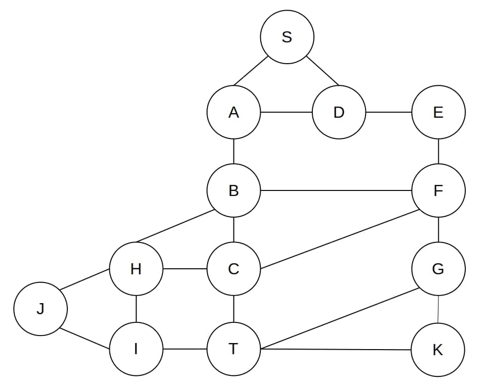
In this example, we want the shortest path from  to
to  . Hence, expanding the children of a node in the proper order, DFS finds the shortest path between and :

Then, it returns ![[T]](/wp-content/ql-cache/quicklatex.com-b046b88ef5231f9f99b3921141fb931a_l3.svg "Rendered by QuickLaTeX.com") to the call in which it expanded
to the call in which it expanded  and prepends to to get
 ![[C, T]](/wp-content/ql-cache/quicklatex.com-71af1fd5ea52e03f71c84ec043c9b37b_l3.svg "Rendered by QuickLaTeX.com") . Furthermore, doing the same with
. Furthermore, doing the same with  and
and  , DFS returns
 ![[A, B, C, T]](/wp-content/ql-cache/quicklatex.com-189121d373d5556ba73bb6998e8ca886_l3.svg "Rendered by QuickLaTeX.com") to the original call, prepends to it, and gives us
to the original call, prepends to it, and gives us ![[S, A, B, C, T]](/wp-content/ql-cache/quicklatex.com-20107a614cc6136376f3232cf47e9f3b_l3.svg "Rendered by QuickLaTeX.com") as the shortest path.
as the shortest path.
In this example, DFS found the shortest path, but if the order in which it visited the children of a node was different, the returned path could be suboptimal.
However, recursive DFS may be slower than the iterative variant:
algorithm IterativeDepthFirstSearch(s, target):
    // INPUT
        s = the start node
        target = the function that identifies a target node
    // OUTPUT
        The target node closest to the start node, or an empty set meaning that no target is reachable

    if target(s):
        return s

    frontier <- a LIFO stack containing only s
    explored <- an empty set

    while frontier is not empty:
        u <- pop the most recently added node from frontier stack
        add u to explored

        for v in neighbors(u):
            if v is not in explored or frontier:
                if target(v):
                    return v
                add v to frontier

    return an empty set
Typically, there are two ways we can trace the path in the iterative DFS. In one approach, after visiting a node, we memorize which node its parent is in the search tree. That way, after finding the target node, we can reconstruct the path by following the parent-child hierarchy. In the other method, we store the full path to each node. Thus, when the search ends, the one leading to the target node is available as well.
Furthermore, we can implement both techniques using different data structures, with or without recursion. However, all the ways work the same, and which one we’ll choose is largely a matter of our preference.
In this case, the key idea is to memorize the parents of the nodes we explore. Let’s say that we expanded a node  and identified its children
  . Hence, for each child, we have to memorize that its parent is :
algorithm IterativeDepthFirstSearchWithPathTracing(s, target, neighbors):
    // INPUT
        s = the start node
        target = the function that identifies a target node
    // OUTPUT
        The shortest path between s and a target node, or empty set meaning that no target is reachable

    if target(s):
        return s

    frontier <- a LIFO stack containing only s
    explored <- an empty set
    memory <- initialize the memory
    Set the parent of s to NULL

    while frontier is not empty:
        u <- pop the most recently added node from frontier stack
        Add u to explored

        for v in neighbors(u):
            Insert the information parent(v) = u into memory

            if v is not in explored or frontier:
                if target(v):
                    path <- reconstruct the path between s and v using memory
                    return path

                Add v to frontier

return empty setFurthermore, to reconstruct the path, we only have to read the memory to get the target’s parent, its parent afterward, and so on, until we reach the start node:
algorithm BackwardPathReconstruction(s, t, memory):
    // INPUT
        s = the start node
        t = the target node found by DFS
        memory = a data structure containing the information on the parent-child relationships
    // OUTPUT
        the shortest path from t to s

    u <- t

    while u != null:
        print u
        u <- find the parent of u in memory
This way, we get the path from the target node to the start node. However, if we want it the other way around, then we should print the path in reverse:
algorithm ForwardPathReconstruction(u, s, t, memory):
    // INPUT
        s = the start node
        t = the target node found by DFS
        memory = a data structure containing the information on the parent-child relationships
    // OUTPUT
        The shortest path from s to t

    path <- an empty LIFO structure
    u <- t

    while u != null:
        push u onto path
        u <- find the parent of u in memory

    while path is not empty:
        u <- pop the node most recently added to path
print uWe can represent the information that  is the parent of
  using different data structures. For example, we can store a pointer to in . Then, reading the memory amounts to traversing a linked list.
Additionally, we can also use hash maps. A common approach is to assign a unique positive integer to each node as its id, treat the ids as indices, and store the parent-child information in an array. Let’s say that  is that array. Thus, the parent of node
  is the node whose id is
 ![memory[i]](/wp-content/ql-cache/quicklatex.com-67f3b44677f08c0f99aca00017900212_l3.svg "Rendered by QuickLaTeX.com") . Hence, its parent is
. Hence, its parent is ![memory[memory[i]]](/wp-content/ql-cache/quicklatex.com-28fe98a5a7917d3000bcdac3bb605d1a_l3.svg "Rendered by QuickLaTeX.com") , and so on.
, and so on.
This is DFS would grow if it expanded the nodes in the order which corresponds to the shortest path between and :
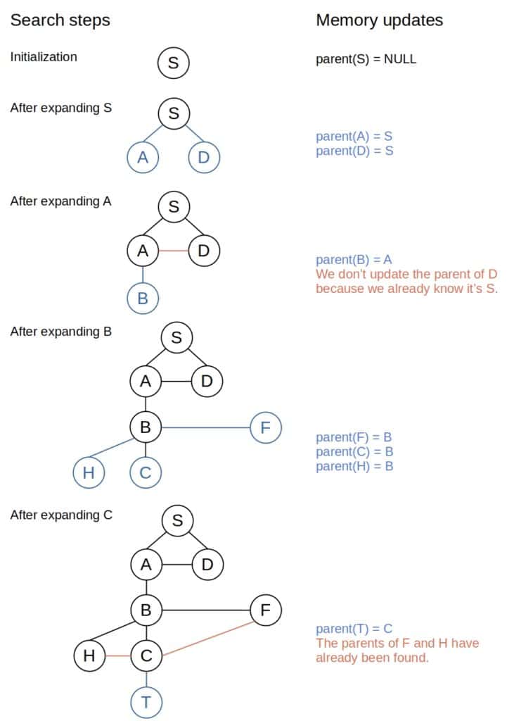
The same comment on the optimality of the path holds in this case.
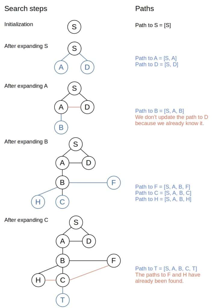
We can also keep track of the paths to the currently active nodes while running DFS. After expanding the node , we remember the paths to the children of  that are its children in the search tree, and once the algorithm identifies a target node, we know we already have the path to it. Therefore, we don’t have to reconstruct it from the memorized information:
algorithm IterativeDFSWithPathMemorization(s, target, neighbors):
    // INPUT
        s = the start node
        target = the function that identifies a target node
    // OUTPUT
        The shortest path between u and a target node

    if target(s):
        return [s]

    frontier <- a LIFO stack containing only (s, [s])
    explored <- an empty set

    while frontier is not empty:
        (u, path_to_u) <- pop from frontier the most recently added pair
        Add u to explored

        for v in neighbors(u):
            path_to_v <- append v to path_to_u
            Insert (v, path_to_v) into memory

            if v is not in explored or frontier:
                if target(v):
                    return path_to_v
                Add (v, path_to_v) to frontier

    return empty set
Thus, this approach is similar to path tracing in the recursive DFS. However, we use more memory because we keep the full paths to all the nodes in the  . In the recursive DFS, we only keep track of one path.
This approach would work like this in the previous example:
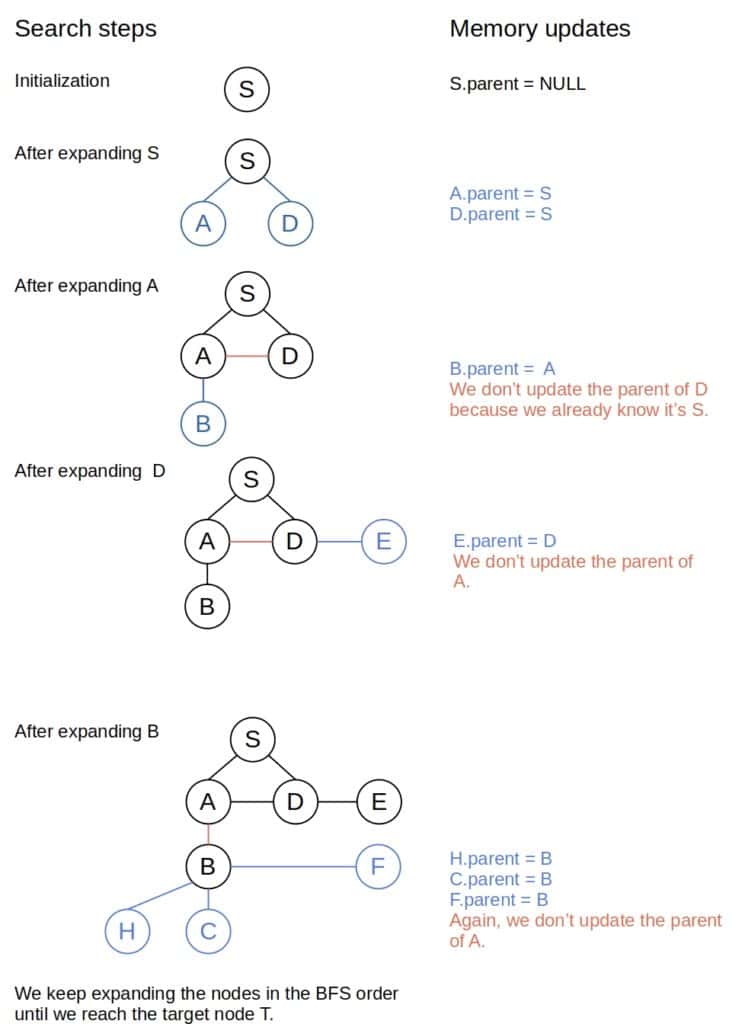
Furthermore, the same approaches that we used for DFS work as well for Breadth-First Search (BFS). However, the only algorithmic difference between DFS and BFS lies in the queue: the former uses a LIFO, whereas the latter uses a FIFO implementation. Moreover, that causes BFS to use way more memory than DFS, so path storing may not be our best option. Instead, we should consider extending the nodes with the pointers to their parents or using a hash map.
That method won’t induce much memory overhead:
algorithm BreadthFirstSearch(s, target, neighbors):
    // INPUT
        s = the start node
        target = the function that identifies a target node
    // OUTPUT
        The shortest path between s and a target node, if one exists.
        Otherwise, the algorithm returns an empty set.

    if target(s):
        return s

    frontier <- a FIFO queue containing only s
    explored <- an empty set
    s.parent <- null
    t <- null

    while frontier is not empty:
        u <- pop the oldest node
        Add u to explored

        for v in neighbors(u):
            v.parent <- u

            if u is not in explored or frontier:
                if target(v):
                    t <- v
                    break
                Add v to frontier

        if target(v):
            break

    if t is null:
        return empty set
    else:
        path <- reconstruct the path from s to t
        return path
Thus, we reconstruct the path just as in Algorithm 5. Additionally, the only thing we should pay attention to is that the line “ find the parent of in ” in Algorithm 5 should be implemented as “
 ” to work with our BFS.
This is how BFS would find the path from to in our example:
Unlike DFS and BFS, Dijkstra’s Algorithm (DA) finds the lengths of the shortest paths from the start node to all the other nodes in the graph. Though limited to finite graphs, DA can handle positive-weighted edges in contrast to DFS and BFS.
Furthermore, we apply the same idea with the memory as before and adapt it to DA. Thus, the algorithm will update the memory as soon as it updates the currently known length of the shortest path between a node in the graph and the start node. Moreover, the array  plays the role of the memory in the pseudocode of DA with path tracing:
algorithm Dijkstra(s, G):
    // INPUT
        s = the start node
        G = a graph
    // OUTPUT
        dist = the lengths of the shortest paths from s to all the other nodes in the graph
        prev = an array such that if prev[j] = i, then the shortest path from s to j finishes with the branch j->i

    queue <- make an empty min-priority queue

    for vertex v in G:
        dist[v] <- infinity
        prev[v] <- null
        Add v to queue with the value infinity

    dist[s] <- 0

    while queue is not empty:
        u <- extract the vertex with the highest priority (minimal value) in queue

        for v in neighbors of u still in the queue:
            alt <- dist[u] + weight(u, v)

            if alt < dist[v]:
                dist[v] <- alt
                prev[v] <- u
                Decrease the priority of v in the queue according to the new value dist[v]

    return (dist, prev)
Thus, using , we can reconstruct the path between and any node  :
:
algorithm BackwardPathReconstruction(s, t, prev):
    // INPUT
        s = the start node
        t = the target node
        prev = the result of Dijkstra's Algorithm
    // OUTPUT
        The shortest path from t to s, if one exists. An empty array otherwise.

    u <- t
    path <- an empty array

    while u != null:
        path <- prepend u to path
        u <- prev[u]

    return path
As we see, it’s the same strategy we used in DFS.
In this article, we showed several ways to trace the paths in Depth-First Search, Breadth-First Search, and Dijkstra’s Algorithm.