

Learn through the super-clean Baeldung Pro experience:
>> Membership and Baeldung Pro.
No ads, dark-mode and 6 months free of IntelliJ Idea Ultimate to start with.
Last updated: March 18, 2024
Learn through the super-clean Baeldung Pro experience:
>> Membership and Baeldung Pro.
No ads, dark-mode and 6 months free of IntelliJ Idea Ultimate to start with.
In this tutorial, we’ll talk about Constraint Satisfaction Problems (CSPs) and present a general backtracking algorithm for solving them.
In a CSP, we have a set of variables with known domains and a set of constraints that impose restrictions on the values those variables can take. Our task is to assign a value to each variable so that we fulfill all the constraints.
So, to formally define a CSP, we specify:


 , where each can involve any number of variables:
![\[C_k: powerset(\mathcal{D}) \rightarrow \{true, false\}\quad k=1,2,\ldots, m\]](/wp-content/ql-cache/quicklatex.com-b291b8cd4495575e6efe25c552c33e0c_l3.svg "Rendered by QuickLaTeX.com")
For example, the squares in a  Sudoku grid can be thought of as variables
 ![S[1,1], S[1,2], \ldots, S[9,8], S[9,9]](/wp-content/ql-cache/quicklatex.com-896737613059dab9e1510e6dd4073bf6_l3.svg "Rendered by QuickLaTeX.com") . The row, column, and block constraints can be expressed via a single relation
. The row, column, and block constraints can be expressed via a single relation  :
:
that’s true if all  are different from one another. Then, Sudoku as a CSP will have
  constraints:
The domains and variables together determine a set of all possible assignments (solutions) that can be complete or partial. Finding the one(s) that satisfy all the constraints is a search problem like finding the shortest path between two nodes in a graph. The CSP search graph’s nodes represent the assignments, and an edge from node  to vertex
  corresponds to a change in a single variable.
The start node is the empty solution, with all variables unassigned. Each time when we cross an edge, we change the value of exactly one variable. The search stops when we find the complete assignment that satisfies all the constraints. The constraint satisfaction check corresponds to the goal test in the general search.
Still, CSPs are not the same as classical search problems. There are two main differences.
First of all, the order in which we set the variables is irrelevant in a CSP. For example, it doesn’t matter if we first set ![S[1,9]](/wp-content/ql-cache/quicklatex.com-1030cdf157458b2c1ea6376430346362_l3.svg "Rendered by QuickLaTeX.com") or
or ![S[9,1]](/wp-content/ql-cache/quicklatex.com-b132f16d50023cbaebfbcc34bb4e93b7_l3.svg "Rendered by QuickLaTeX.com") in solving Sudoku. In contrast, the order does matter when searching for the shortest path between two points on a map. We first have to get from point
in solving Sudoku. In contrast, the order does matter when searching for the shortest path between two points on a map. We first have to get from point  to
to  before going from to
  . So, a solution to a classical search problem is an ordered sequence of actions, whereas a solution to a CSP is a set of assignments that we can make in any order we like.
The second difference is that the solutions in classical search are atomic from the algorithms’ point of view. They apply the goal test and cost function to solutions but don’t inspect their inner structures. On the other hand, the algorithms for solving CSPs know the individual variables that make the solution and set them one by one.
We can visualize the CSP and the structure of its solutions as a constraint graph. If all the constraints are binary, the nodes in the graph represent the CSP variables, and the edges denote the constraints acting upon them.
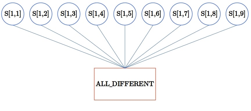
However, if the constraints involve more than two variables (in which case, we call them global), we create constraint hyper-graphs. They contain two types of nodes: the regular nodes that represent variables and hyper-nodes that represent constraints. For instance, Sudoku has 9-ary constraints. So, a part of its hyper-graph would look like this:
A constraint can be unary, which means that it restricts a single variable. A CSP with only unary and binary constraints is called a binary CSP. By introducing auxiliary variables, we can turn any global constraint on finite-domain variables into a set of binary constraints. So, it seems that we can focus on binary CSPs and that there’s no need to develop solvers that consider higher-order constraints.
However, it can still pay off to work with global constraints. The reason is that a restriction such as is more easily implemented and understood than a set of binary constraints. Additionally, the solvers that exploit the specifics of a global constraint can be more efficient than those which operate only on binary and unary constraints.
Here, we’ll present the backtracking algorithm for constraint satisfaction. The idea is to start from an empty solution and set the variables one by one until we assign values to all. When setting a variable, we consider only the values consistent with those of the previously set variables. If we realize that we can’t set a variable without violating a constraint, we backtrack to one of those we set before. Then, we set it to the next value in its domain and continue with other unassigned variables.
Although the order in which we assign the variables their values don’t affect the correctness of the solution, it does influence the algorithm’s efficacy. The same goes for the order in which we try the values in a variable’s domain. Moreover, it turns out that whenever we set a variable, we can infer which values of the other variables are inconsistent with the current assignment and discard them without traversing the whole sub-tree.
With that in mind, we present the pseudocode:
algorithm BacktrackingForConstraintSatisfaction(csp):
    // INPUT
    //    csp = the definition of the CSP to solve by recursively traversing its search tree
    // OUTPUT
    //    an assignment of variables that satisfies the constraints, or failure if no solution exists

    assignment <- make an empty assignment
    return BACKTRACK(csp, assignment)

algorithm BACKTRACK(csp, assignment):
    // INPUT
    //    csp = the definition of the CSP to solve
    //    assignment = the current assignment of variables
    // OUTPUT
    //    an assignment of variables that satisfies the constraints, or failure if no solution exists

    if assignment is complete:
        return assignment

    var <- SELECT-UNASSIGNED-VARIABLE(csp, assignment)

    for value in ORDER-VALUES(csp, var, assignment):
        if value is consistent with assignment:
            add {var = value} to assignment
            inferences <- INFERENCE(csp, var, assignment)

            if inferences != failure:
                add inferences to csp
                result <- BACKTRACK(csp, assignment)

                if result != failure:
                    return result

                remove inferences from csp

            remove {var = value} from assignment

    return failure
The way we implement variable selection, value ordering, and inference is crucial for performance. In traditional search, we improved the algorithms by formulating problem-specific heuristics that guided the search efficiently. However, it turns out that there are domain-independent techniques we can use to speed up the backtracking solver for CSPs.
Let’s talk about inference first. That’s a step we make right after setting a variable  to a value
  in its domain. We iterate over all the variables connected to
  in the constraint (hyper)graph and remove the values inconsistent with the assignment
  from their domains. That way, we prune the search tree as we discard impossible assignments in advance. This technique is known as forwarding checking. However, we can do more.
Whenever we prune a value from  , we can check what happens to the neighbors of
  in the graph. More specifically, for every
  that is connected to via a constraint
  , we check if there’s a value
  such that
  satisfies
  only if
  . Any such value
  can be discarded because any assignment containing is impossible too. However, this assumes that all the constraints are binary.
A straightforward strategy for variable selection is to consider the variables in a static order we fix before solving the CSP at hand. Or, we may select the next variable randomly. However, those aren’t efficient strategies. If there’s a variable with only one value in its domain, it makes sense to set it before others. The reason is that it optimizes the worst-case performance.
In the worst-case scenario, we can’t complete the current partial assignment, so the backtracking search will return  after traversing the whole sub-tree under that assignment. But, the variable with only one legal value is the most likely to conflict with other variables at shallower levels of the sub-tree and reveal its inconsistency. In general, this is the rationale for the Minimum-Remaining-Values heuristic (MRV). MRV chooses the variable with the fewest legal values remaining in its domain.
The value ordering heuristic follows the opposite logic. When setting to a value, we should choose the one that rules out the fewest values from the domains of the ‘s neighbors. The intuition behind this choice is that we need only one solution, and it’s more likely for a larger sub-tree to contain it than for a smaller one. We call this strategy the Least-Constraining-Value heuristic (LCV).
In a way, LCV balances off the tendency of MRV to prune the search tree as much as possible. CSP solvers that incorporate both heuristics are usually very efficient in practice. However, we should note that MRV doesn’t require the CSP to be binary, whereas LCV does. That’s not a problem because we can convert any CSP to a binary form. However, if we use custom-made inference rules that operate on higher-order constraints such as , we should make sure to maintain both representations of the CSP during the execution of the backtracking solver.
In this article, we presented a general backtracking algorithm for solving constraint satisfaction problems. We also talked about some heuristic strategies to make the solver more efficient.
![\[ALL\_DIFFERENT(x_1, x_2, \ldots, x_n)\]](/wp-content/ql-cache/quicklatex.com-9f8b696c2ae69850dca3db2a4f028889_l3.svg "Rendered by QuickLaTeX.com")
![\[\begin{aligned} \\ &\text{9 row constraints:} \\ &(\forall i=1,2,\ldots, 9)&& ALL\_DIFFERENT(S[i,1], S[i,2], \ldots, S[i, 9]) \\ &\text{9 column constraints:} \\ &(\forall j=1,2,\ldots, 9) &&ALL\_DIFFERENT(S[1,j], S[2,j], \ldots, S[9, j]) \\ &\text{and 9 block constraints:}\\ & && ALL\_DIFFERENT(S[1, 1], S[1, 2], S[1, 3], S[2, 1], \ldots, S[3, 3]) \\ & && ALL\_DIFFERENT(S[1, 4], S[1, 5], S[1, 6], S[2, 4], \ldots, S[3, 6]) \\ & \ldots && \\ & && ALL\_DIFFERENT(S[7, 7], S[7, 8], S[7, 9], S[8, 7], \ldots, S[9, 9]) \\ \end{aligned}\]](/wp-content/ql-cache/quicklatex.com-bd7857726fedd7464f930272476fdf1c_l3.svg "Rendered by QuickLaTeX.com")