

Learn through the super-clean Baeldung Pro experience:
>> Membership and Baeldung Pro.
No ads, dark-mode and 6 months free of IntelliJ Idea Ultimate to start with.
Last updated: December 10, 2025
Learn through the super-clean Baeldung Pro experience:
>> Membership and Baeldung Pro.
No ads, dark-mode and 6 months free of IntelliJ Idea Ultimate to start with.
CPU scheduling is a crucial feature of operating systems that govern sharing processor time among the numerous tasks running on a computer. Hence, it is essential to ensure efficiency and fairness in executing processes. It also ensures that the system can fulfill its users’ performance and responsiveness requirements.
CPU scheduling comprises many essential concepts.
In this tutorial, we’ll discuss concepts central to CPU scheduling, including arrival, burst, completion, turnaround, waiting, and response time. By understanding these concepts and how they are used in different scheduling algorithms, we can gain a deeper understanding of how operating systems manage the execution of processes on a computer.
In CPU Scheduling, the arrival time refers to the moment in time when a process enters the ready queue and is awaiting execution by the CPU. In other words, it is the point at which a process becomes eligible for scheduling.
Many CPU scheduling algorithms consider arrival time when selecting the next process for execution. A scheduler, for example, may favor processes with earlier arrival timings over those with later arrival times to reduce the waiting time for a process in the ready queue. Hence, it can assist in ensuring the execution of processes efficiently.
Burst time, also referred to as “execution time”. It is the amount of CPU time the process requires to complete its execution. It is the amount of processing time required by a process to execute a specific task or unit of a job. Factors such as the task’s complexity, code efficiency, and the system’s resources determine the process’s burst time.
The burst time is also an essential factor in CPU scheduling. A scheduler, for example, may favor processes with shorter burst durations over those with longer burst times. This will reduce the time a process spends operating on the CPU. Hence, it can assist in ensuring that the system can make optimum use of the processor’s resources.
Completion time is when a process finishes execution and is no longer being processed by the CPU. It is the summation of the arrival, waiting, and burst times.
Completion time is an essential metric in CPU scheduling, as it can help determine the efficiency of the scheduling algorithm. It is also helpful in determining the waiting time of a process.
For example, a scheduling algorithm that consistently results in shorter completion times for processes is considered more efficient than one that consistently results in longer completion times.
The time elapsed between the arrival of a process and its completion is known as turnaround time. That is, the duration it takes for a process to complete its execution and leave the system.
Turnaround Time = Completion Time – Arrival TimeA scheduling algorithm that regularly produces shorter turnaround times for processes is considered more efficient than one with longer turnaround times.
This is a process’s duration in the ready queue before it begins executing. It helps assess how efficient the scheduling algorithm is. A scheduling method that consistently results in reduced wait times for processes, for example, is considered more efficient than one that regularly results in longer wait times.
Waiting Time = Turnaround Time – Burst TimeFurthermore, it helps to measure the efficiency of a scheduling algorithm. Also, it aids in determining a system’s perceived responsiveness to user queries. A long wait time can contribute to a negative user experience. This is because consumers may view the system as slow to react to their requests.
Response time is the amount of time it takes for the CPU to respond to a request made by a process. It is the duration between the arrival of a process and the first time it runs. It is an essential parameter in CPU scheduling since it may assist in determining a system’s perceived responsiveness to user requests.
Response Time = Time it Started Executing – Arrival TimeThe number of processes waiting in the ready queue, the priority of the processes, and the features of the scheduling algorithm are all variables that might impact response time. For example, a scheduling algorithm that prioritizes processes with shorter burst times may result in quicker response times for those processes.
To further illustrate this concept and how they are calculated, let’s consider an example with four processes as shown in the table, including arrival time and burst time. Using the non-preemptive shortest-job-first algorithm, we can see how the processes are completed:
| Process | Arrival Time | Burst Time |
|---|---|---|
| P1 | 3 | 3 |
| P2 | 6 | 3 |
| P3 | 0 | 4 |
| P4 | 2 | 5 |
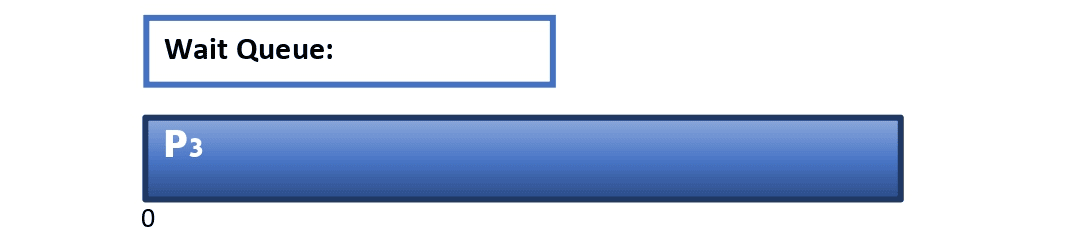
At time=0: P3 arrives and starts execution without waiting.
Let’s note that P3 is first attended to at time=0:
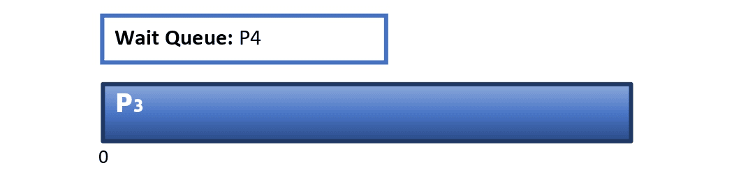
At time=2: P4 arrives, and P3 continues executing.
Hence, P4 waits in the queue:
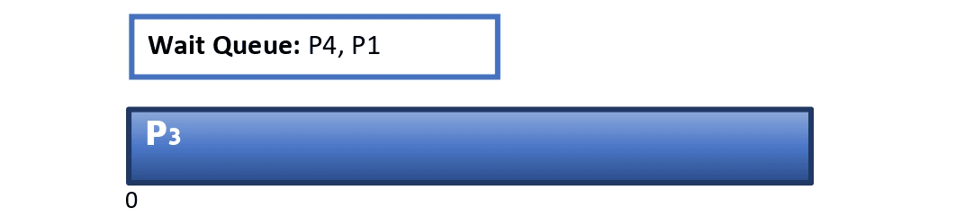
At time=3: P1 arrives, and P3 continues executing:
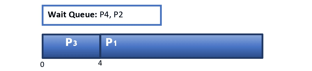
At time=4: P3 completes execution. The burst time for P4 and P1 are compared. Hence P1 starts executing:
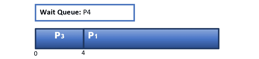
At this point, we can calculate the Turnaround, Wait, and Response Time for P3:
Completion Time (P3) = 4
Turnaround Time (P3) = 4 - 0 = 4
Wait time (P3) = 4 - 4 = 0
Response Time (P3) = 0 - 0 = 0
At time=6: P2 arrives, and P1 is still executing:
At time=7: P1 completes execution. The burst time for P4 and P2 are compared. Hence, P2 starts executing:

Now, we can make calculations for P1:
Completion Time (P1) = 7
Turnaround Time (P1) = 7 - 3 = 4
Wait time (P1) = 4 - 3 = 1
Response Time (P1) = 4 - 3 = 1
At time=10: P2 completes execution, and only P4 is in the wait queue. Hence, P4 starts executing:

At this point, we can make calculations for P2:
Completion Time (P2) = 10
Turnaround Time (P2) = 10 - 6 = 4
Wait Time (P2) = 4 - 3 = 1
Response Time (P2) = 7 - 6 = 1
At time=15: P4 completes execution. Hence, we have the Gantt Chart:
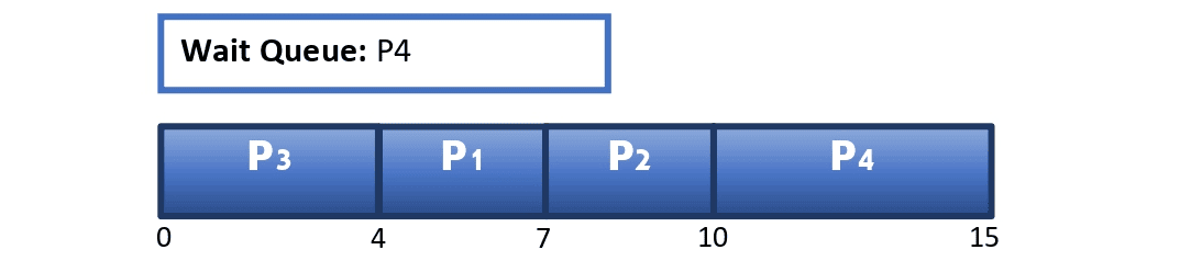
We can now make calculations for P4:
Completion Time (P4) = 15
Turnaround Time (P4) = 15 - 2 = 13
Wait Time (P4) = 13 - 5 = 8
Response Time (P4) = 10 - 2 = 8This article discussed CPU scheduling concepts: arrival, burst, completion, turnaround, waiting, and response times. We also discussed how to calculate them, providing an example for illustration.
By taking these elements into account, operating systems may efficiently balance the demands of various activities to enhance the system’s overall performance and efficiency.