

Learn through the super-clean Baeldung Pro experience:
>> Membership and Baeldung Pro.
No ads, dark-mode and 6 months free of IntelliJ Idea Ultimate to start with.
Learn through the super-clean Baeldung Pro experience:
>> Membership and Baeldung Pro.
No ads, dark-mode and 6 months free of IntelliJ Idea Ultimate to start with.
We often study how one variable influences another. For example, we may want to determine if older persons have more chances of having pneumonia than younger ones or find out how house prices vary depending on the number of bedrooms.
In this tutorial, we’ll discuss two statistical concepts: correlation and regression. Although they share the goal of studying the relationship between variables, they have different approaches and applications.
A correlation coefficient quantifies the strength of association between two variables and indicates the direction of their relationship.
For example, the Pearson coefficient  ranges from -1 to +1. When is close to 1, we have a positive and strong linear relationship between the variables: if one variable increases, the other will also increase.
On the other hand, as approaches -1, we have a strong negative linear relationship. This means that if one of the variables increases, the other decreases. Finally, a correlation coefficient equal to zero indicates no linear relationship between the variables.
Studying nonlinear dependencies between variables requires a more complex analysis, so we won’t cover them in this article. We have Spearman’s rank correlation and Kendall’s tau coefficients as examples of coefficients capable of capturing nonlinear relationships.
Regression estimates the functional relationship between the dependent and independent variables.
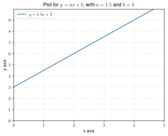
In the case of linear regression, we get a line fitted to the original data. The regression equation describes this line:
![\[y = ax + b\]](/wp-content/ql-cache/quicklatex.com-ecb7e10cd2d56525d129325e2efc0573_l3.svg "Rendered by QuickLaTeX.com")
So, linear regression finds the equation for computing the dependent variable  from the independent variable
  . In this equation, the value of
  indicates the slope of the line, and
  indicates the point where the line intercepts the axis:
Furthermore, the regression can handle the case with multiple independent variables  :
:
![\[y = \alpha_0 + \alpha_1 x_1 + \alpha_2 x_2 + \ldots + \alpha_m x_m\]](/wp-content/ql-cache/quicklatex.com-e01d1e430becc4c29771308549f92164_l3.svg "Rendered by QuickLaTeX.com")
In this equation,  represents the y-intercept when all independent variables equal zero. Each
  represents the change in relative to a change in
  .
.
We can also fit nonlinear functions, e.g.:
![\[y = a x^2 + b x + c\]](/wp-content/ql-cache/quicklatex.com-509c13840ad0127b26504ab847c424f2_l3.svg "Rendered by QuickLaTeX.com")
To do so, we need to choose the form of functional relationship before fitting.
We’ll show the difference between correlation and regression with two examples.
In the first scenario, we’ll consider the children’s age as the independent variable and average height as the dependent variable:
| Age (month) | Height (cm) |
|---|---|
| 18 | 76.1 |
| 19 | 77.0 |
| 20 | 78.1 |
| 21 | 78.2 |
| 22 | 78.8 |
| 23 | 79.7 |
| 24 | 79.9 |
| 25 | 81.1 |
| 26 | 81.2 |
| 27 | 81.8 |
| 28 | 83.5 |
First, let’s calculate the Pearson correlation coefficient. For this data, we get  . This indicates, as expected, that height increases with age. Or in other words, the two variables have a strong and positive linear relationship.
But what if we want to estimate the expected height for a 32-month-old or find the mathematical form of the relationship?
For that, we need regression. The linear regression gives us the following:
![\[height = 0.6263 age + 65.1118\]](/wp-content/ql-cache/quicklatex.com-4963f2c51e9e7325c99664232dd3951a_l3.svg "Rendered by QuickLaTeX.com")
Visually:
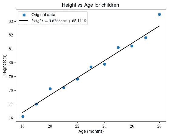
Although we couldn’t perfectly fit the regression line to the data, it’s clear that the fit is satisfactory.
By setting  , we obtain
  .
.
Let’s say we want to model the trajectory of a ball after it a throw. Our independent variable is the time in seconds, and our dependent variable is the height in centimeters:
| Time (s) | Height (cm) |
|---|---|
| 0 | 0.0 |
| 1 | 3.5 |
| 2 | 7.0 |
| 3 | 8.5 |
| 4 | 7.0 |
| 5 | 3.5 |
| 6 | 0.0 |
Let’s start by computing the Pearson correlation coefficient. Then, we find that  , which indicates that there is no linear relationship between the two studied variables. However, we’ll see a clear quadratic relationship if we plot the data and fit a (quadratic) model:
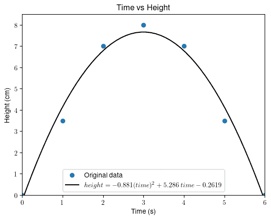
Since we have a nonlinear and non-monotonic relationship, the traditional correlation coefficients won’t provide any insights into the data.
If we had a strictly increasing or decreasing behavior (i.e., monotonic), Spearman’s or Kendall’s tau coefficients would easily prove the correlation between them.
Let’s summarize the main differences between correlation and regression.
| Correlation | Regression |
|---|---|
| A number | A model (formula) |
| Shows the strength of the relationship | Describes the relationship between dependent and independent variables |
| Can’t predict new values | Can estimate the dependent variable for any valid value of the independent variable |
| Requires complex analysis for nonlinear and non-monotonic cases | Polynomial regression can usually handle nonlinear cases |
In this article, we discussed correlation and regression. They provide different ways of analyzing the relationship between variables.
A correlation coefficient is a number that indicates how strongly two variables are related. In contrast, regression describes the relationship with an actual equation we can use to estimate the value of the dependent variable.
We should remember that these are tools that can be used together. Once we start working with some data, we can compute the correlation coefficient first. If it’s strong, we can invest more time in fitting a linear model to the data.