How to Reduce/Extend 2-D Convolutions to 1-D and 3-D?

1. Introduction

When we hear about convolutions in machine learning and deep neural networks, we typically think about 2-D convolutions used for image recognition tasks. Indeed, convolutional neural networks (CNNs) revolutionized the field of computer vision by learning filters directly from images. However, these same principles extend naturally to spaces with different dimensionalities. For example, we can apply convolutions to 1-D signals like audio data or time series and 3-D volumetric data, such as MRI scans or video frames.

So, how exactly do we adapt the familiar 2-D convolution to 1-D or 3-D? The mechanics of sliding filters to compute weighted sums (the definition of convolution) remain the same. We only change how we move the kernel.

In this tutorial, we’ll explore the conceptual similarities and differences among 1-D, 2-D, and 3-D convolutions. By the end, we’ll have a practical understanding of transferring the same convolutional logic across multiple data shapes.

2. Basic Concepts of Convolution

A convolution is a mathematical operation that slides a kernel (or filter) across input data, computing dot products at each position. This dot product often involves a small window of input elements and corresponding filter weights.

After an entire pass, we get new values (often called feature maps in deep learning).

Let’s review the basics of 2-D convolution.

2.1. 2-D Convolution Overview

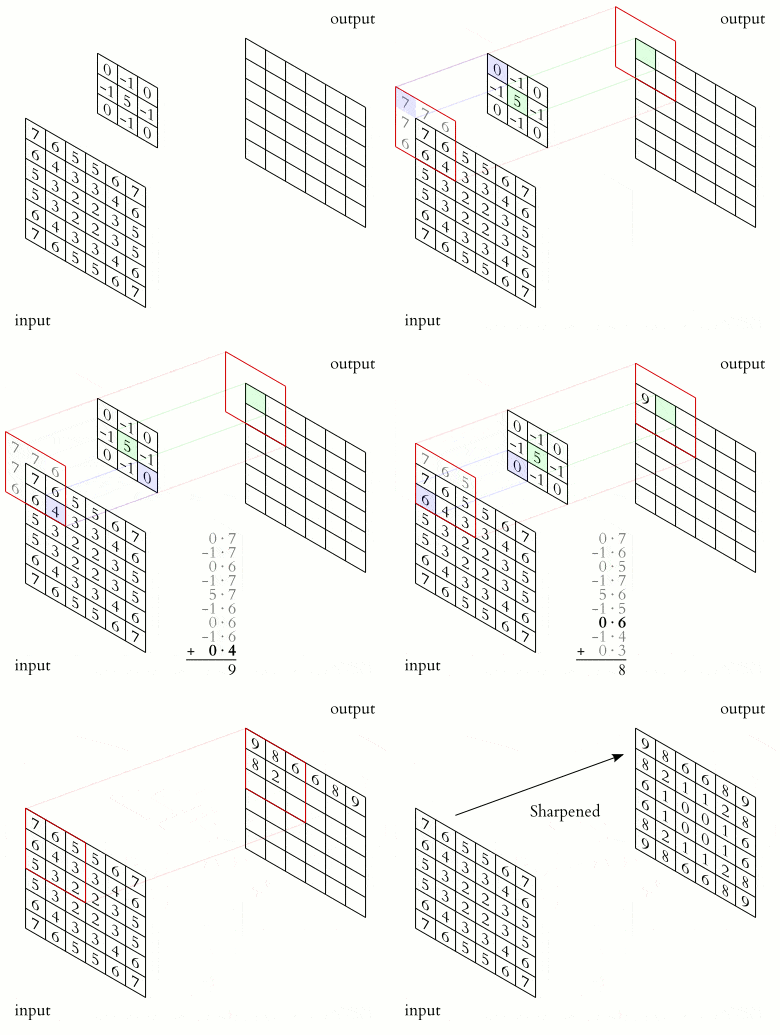
2-D convolution is perhaps the most famous type due to image processing. Here, the kernel is a 2-D grid of weights, e.g., 3×3 or 5×5. It slides over the image, computing the output values using this formula:

Here, (i, j) are the spatial coordinates in the output, and (m, n) indexes the kernel coordinates. In practice, frameworks like PyTorch or TensorFlow handle computation, but this formula underpins how CNNs learn to detect features such as edges or textures in images.

Geometrically, we perform these steps:

1. align the kernel’s top-left corner with the pixel at (i, j)
2. multiply each kernel weight by the corresponding input pixel in the overlapped region
3. sum these products to produce the output at Output(i,j)
4. slide the kernel, typically by a stride in the horizontal direction, moving left to right, top to bottom, and compute the output at that new position in the same way

Visually:

When dealing with color images, we have multiple channels (e.g., RGB = 3). The kernel will have a matching depth (also 3) to sum across all channels.

2.2. Why Do We Use Convolutions?

Convolutions are useful because they:

• capture local patterns: the kernel is smaller than the entire input, focusing on local neighborhoods
• are parameter-efficient: the same kernel weights are reused at every position, which drastically reduces the number of parameters compared to fully connected layers
• preserve the structure (spatial, temporal, or volumetric): by sliding across input dimensions, we retain the relationships in the original data

3. The Case for 1-D Convolution

When dealing with sequential input, such as audio data, stock prices, sensor readings, or language tokens, we use convolutional filters that work in one dimension. So, instead of scanning across a 2-D grid, we shift a 1-D kernel over a single axis.

3.1. What Is 1-D Convolution?

In 1-D convolution, we define the output as:

Here, Input is a 1-D array, such as amplitudes over time or some numeric feature over an index. The kernel has a small width, often called the kernel size (), and iterates over 1 to . We slide the kernel from the start to the end of the signal.

A typical usage might be applying a kernel of size three that picks up local patterns in the sequence, such as a wave pattern in an audio clip or a short-time feature in a sensor reading.

3.2. PyTorch Example

Let’s say we have a 1-D array of amplitude values over time steps that we want to use in audio processing. A 1-D convolution slides a small filter across the time axis to detect short bursts of frequencies or wave shapes, much like 2-D filters detect edges or shapes in images.

In the torch framework for deep learning, we use the Conv1d layer to define a one-dimensional kernel:

import torch
import torch.nn as nn

# Example: 1-D convolution layer in PyTorch
conv1d_layer = nn.Conv1d(in_channels=1, out_channels=8, kernel_size=3, stride=1)

Here:

• in_channels=1 means there’s a single channel
• out_channels=8 means we learn 8 different filters
• kernel_size=3 means each filter sees three adjacent time steps
• stride=1 means we slide the window in each step by one item in the input sequence

Just like images can have RGB channels, 1-D signals can have multiple channels. Examples are multi-sensor data and stereo audio signals. To accommodate such data, we define in_channels > 1. The convolution is still 1-D in structure, but it spans across however many input channels exist for each time step.

Below is an example where we simulate some dummy data and apply the layer conv1d_layer we previously created:

# Create dummy audio data with shape (batch=4, channels=1, length=100)
audio_data = torch.randn(4, 1, 100)

# Pass data through the 1-D convolution layer
output_1d = conv1d_layer(audio_data)
print("1D output shape:", output_1d.shape)

4. Overview of 3-D Convolution

Now, let’s move to the next dimension: 3-D data.

One significant use case is volumetric data, such as CT or MRI scans, where each “pixel” is actually a voxel in a 3-D space. Another example is video data, where we treat frames as the time dimension on top of 2-D images.

4.1. Defining the 3-D Kernel

A 3-D convolution layer uses a 3-D kernel, e.g., kernel_size=(3,3,3). We slide this kernel in three axes. Let (x, y, z) denote those axes. The convolution operation is then:

We add up the products of overlapped cells in 3-D space. By scanning across the volume, we produce a 3-D output (or 4-D if we include multiple filters/channels because, in that case, each 3-D point is actually a vector). Here’s a visualization:

4.2. PyTorch Example

In many medical tasks (e.g., tumor segmentation and 3-D organ detection), we load volumetric scans.

Here’s how we define a 3-D convolution in PyTorch:

import torch
import torch.nn as nn

conv3d_layer = nn.Conv3d(in_channels=1, out_channels=8, kernel_size=(3,3,3), stride=1)

Here:

• in_channels=1 sets a single volumetric channel (like a single MRI sequence)
• out_channels=8 means we learn eight filters in the 3-D space
• kernel_size=(3,3,3) indicates the kernel is a 3×3×3 cube

If we consider a short video as a 3-D arrangement of frame width height (not counting color channels), we can slide the convolution across space and time. This yields spatiotemporal features, letting a model detect spatial patterns and how they evolve over time. Some video action recognition architectures rely on 3-D convolution to capture these dynamic spatiotemporal cues.

Let’s see how to apply the layer conv3d_layer:

# Create dummy volumetric data (batch=2, channels=1, depth=10, height=64, width=64)
volume_data = torch.randn(2, 1, 10, 64, 64)

# Pass data through the 3-D convolution layer
output_3d = conv3d_layer(volume_data)
print("3D output shape:", output_3d.shape)

5. Data Shapes

Convolution in 2-D is often our starting point (especially in computer vision tasks). 3-D convolution is like 2-D with an extra dimension, and 1-D is like 2-D without one dimension:

• 2-D uses a two-dimensional kernel, so it expects (m,n) as the kernel (window) size
• 1-D replaces (m,n) with k
• 3-D replaces (m,n) with (p,q,r)

The core sliding dot product operation remains conceptually the same in all three cases. The only change is the number of dimensions, which affects the expected data shape.

With batching, the data should have the following shape in PyTorch:

• (batch_size, number_of_channels, length) in 1-D
• (batch_size, number_of_channels, height, width) in 2-D
• (batch_size, number_of_channels, depth, height, width) in 3-D

This means we can use the same settings for the parameters such as in_channels, out_channels, kernel_size, etc., in 1-D, 2-D, and 3-D applications.

However, didn’t we say the kernel sizes differ in these three cases? For example, would it be a mistake to use kernel_size=3 in 2-D or 3-D? In PyTorch, the kernel size can be an integer, but then it’s expanded to a tuple with the correct number of dimensions. So, kernel_size=3 in 2-D is shorthand for (3,3), and in 3-D, kernel_size=3 expands to (3,3,3). If we want other expansions, e.g., 3 to (3, 1) or (1, 3) in 2-D, we should set this parameter explicitly. This holds for the following parameters as well:

• stride = how much the kernel window moves between steps
• dilation = “the spacing between kernel points“

6. Performance and Practical Considerations

6.1. Memory Usage

Because of its size, 3-D convolution is slower than 2-D convolution, which is, in turn, slower than 1-D convolution.

For example, when a 3-D CNN handles large volumes, that means more computations per forward pass and more data stored in memory for activations. As a result, we often need to use small batches or scale GPU resources accordingly.

6.2. Kernel Size Selection

In 1-D signals, we’d want to pick smaller kernel sizes (3, 5, or 7) to capture local patterns. In 3-D, a typical kernel is (3×3×3). For images, 3×3 or 5×5 are common. The exact size depends on the application, but as said for 1-D convolution, smaller kernels are likely to focus on local patterns successfully.

On the other hand, larger kernels (like 7×7 or 11×11) are used sometimes, but they significantly increase computations, so modern architectures often rely on multiple small kernels stacked together.

6.3. Stride and Dilation

We can adjust the stride to skip certain positions, effectively downsampling. Alternatively, we can increase dilation to see a broader range while using fewer weights.

These are advanced tweaks that help tune the receptive field. For example, dilated convolutions can help reveal wider contexts without increasing kernel size.

6.4. Handling Edge Cases

Padding is crucial. In 2-D, we typically do “same” padding to preserve spatial size.

By “same” padding, we mean that the output’s dimensions match the input’s dimensions, ensuring the convolution doesn’t reduce the feature map size along the data axes.

In 1-D or 3-D, we might want the “same” logic if we don’t want the output to shrink. Each library has slightly different defaults, so we must confirm we’re consistent with our target architecture.

7. Comparison of 1-D, 2-D, and 3-D Convolutions

In practice, 1-D, 2-D, and 3-D convolutions work on the same principle: a sliding window dot product over the input. However, they differ in how many axes they convolve over and in the tasks they commonly address.

Below is a table summarizing typical input shapes, kernel sizes, and use cases across these three convolution types:

8. Conclusion

In this article, we focused on convolutions that form the backbone of many deep learning architectures. While most well-known for handling 2-D images, they naturally generalize to 1-D signals (like audio and time series) and 3-D volumes (like medical scans or video clips).

The difference is in how we move the kernel across input dimensions: in 1-D, we shift along only one axis, while in 3-D, we shift along three, capturing volumetric or spatiotemporal patterns. To see more of the changes and how they affect visually the dimensions (e.g., in CNN), please refer to this article.