

Yes, we're now running our only Summer Sale. All Courses are 30% off until 20th July, 2026:
Big-O Notation of Stacks, Queues, Deques, and Sets
Last updated: March 18, 2024
Learn through the super-clean Baeldung Pro experience:
>> Membership and Baeldung Pro.
No ads, dark-mode and 6 months free of IntelliJ Idea Ultimate to start with.
1. Overview
In this tutorial, we’ll explain the complexities of operations on the main data structures like stacks, queues, deques, and sets. For each of them, we’ll shortly list the main operations and explain the complexity behind them.
2. Stacks
The stack data structure supports the operations of adding and retrieving elements in a LIFO order (Last In, First Out). This term refers to the fact that new elements are added to the beginning of the stack, and the first element to be retrieved is the last added element.
The complexity of these operations varies depending on the implementation. The most efficient way to implement a stack is using a simple linked list. Thus, we’ll discuss the complexity of each operation, assuming the stack is implemented using a linked list.
Take a look at the figure showing the general overview of a stack:
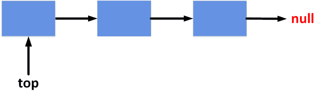
The list is controlled by referencing the first element, usually the top.
2.1. Add an Element
Adding an element to a stack is usually called a  operation. The operation is simply done by adding a new element before the
  and changing the top element to become the newly added one.
The complexity of such an operation is  because we only do constant timing operations.
2.2. Remove an Element
Removing an element from the top of the stack is called a  operation. It’s achieved by moving the reference one step forward to the next element. Thus, the time complexity of this operation is also .
2.3. Get an Element
In stacks, we usually want to know the value of the top element. This operation is simply done by retrieving the value of the element referenced by the pointer. Thus, it has a constant time complexity equal to .
2.4. Check Emptiness
When we want to check whether the stack contains any elements or not, we can check whether the reference points to  or not. If so, the stack is empty. Otherwise, it has at least one element. This check can be implemented in an time complexity.
3. Queues
Queues support the operation of lining up elements one after the other. All new elements are added to the end of the queue, while the first element to be retrieved from the queue is the first added element. This is also known as FIFO (First In, First Out).
Similar to stacks, the most efficient way to implement queues is using linked lists. However, since adding and retrieving elements happen from two different ends of the list, we use two pointer references to hold the first and last elements. The following shape describes the general overview of a queue:
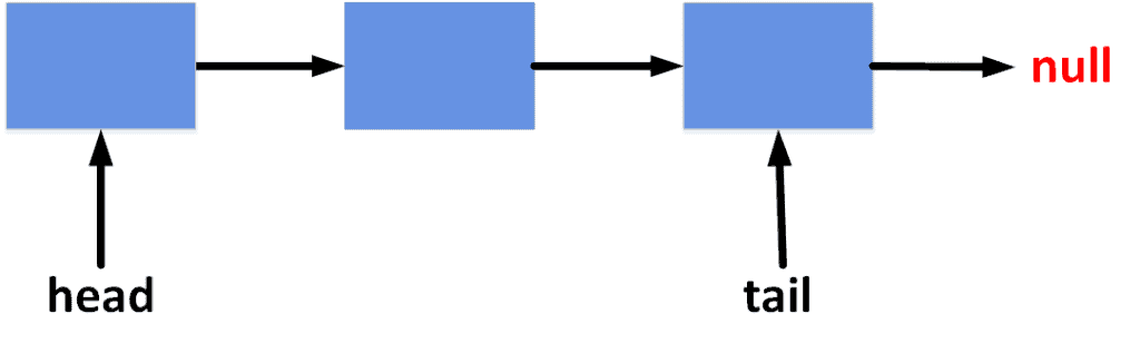
We can call the reference to the first element the  , while the reference to the last one is the
  . Note that, in a queue, each element points to the next one to make it easier to support adding and removing elements.
3.1. Add an Element
Similar to a stack, the operation of adding an element to a queue is called a operation. It can be achieved by adding the new element after the reference and moving the to point to the newly added element. Since the operation is achieved by moving references with a constant time, the overall complexity is .
3.2. Remove an Element
As described, we remove elements from the beginning of the queue. This is done by moving the reference one step forward and deleting the element that was excluded from the queue. We can implement the operation in time complexity.
3.3. Get an Element
Since we are always interested in the element at the beginning of the queue, we need to return the value of the element that is pointed to by the reference. This operation has a time complexity of .
3.4. Check Emptiness
Checking whether a queue is empty is done by checking the value of either the or references. If they point to , then it means the queue is empty. Implementing this check is done with time complexity.
4. Deques
Deques mix the behavior of stacks and queues. We can add elements to the beginning and end of a deque. Plus, we can retrieve elements from either end. To achieve this, we can implement deques using a double-linked list. Take a look at the following diagram to get an idea of the general structure of deques:
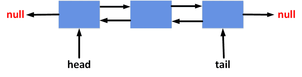
We have two pointer references called and , which allow us to add and delete elements from both ends.
4.1. Add an Element
As described, we can add elements to the beginning and end of a deque. These operations are usually called  and
and  . We can implement them by adding an element before the or after the and moving the corresponding references.
Since it’s just moving pointer references, the overall complexity is .
4.2. Remove an Element
We can remove elements from both ends with operations called  and
and  . This is done by moving the pointer one step forward or the pointer one step backward. Thus, the time complexity is .
4.3. Get an Element
We can get either the first or last element from a deque by getting the value of the element at the position of the or references. The time complexity for such operations is .
4.4. Check Emptiness
To check whether a deque is empty, it is enough to check whether the or is . If so, then the deque is empty. This can be done in time complexity.
5. Sets
Sets data structures are more complex than stacks, queues, and deques. We have two types of sets. Either it is an ordered set, which keeps the elements sorted, or a hash set, which hashes the elements to make it easier to find them. As a reminder, sets only allow each element to be added once.
Ordered sets are usually implemented with red-black trees to support the main operations in logarithmic time complexity. On the other hand, hash sets are implemented using the hash table data structure.
5.1. Add an Element
In the case of an ordered set, adding an element has a time complexity of  , where
  is the number of elements already in the set. This is because red-black trees have to keep the elements sorted.
Since hash sets rely on hash tables, the complexity is constant. In general, the complexity is close to .
5.2. Remove an Element
To remove an element from an ordered set, the red-black tree has to remain sorted. Thus, the complexity for ordered sets is , where is the number of elements in the set. Hash sets, however, only need to hash the element to find and remove it. Therefore, the complexity for hash sets is .
5.3. Get an Element
To find an element in an ordered set, we need time complexity, where is the number of elements in the set. However, with hash sets, we can quickly find the element by hashing its value. Hence, the complexity for hash sets is .
5.4. Check Emptiness
Checking if the set is empty or not has a constant time complexity for both ordered sets and hash sets. The complexity in both cases is .
6. Comparison
The following table summarizes a comparison between the complexities in different data structures:
| Add | Remove | Retrieve | Emptiness | |
|---|---|---|---|---|
| Stacks | O(1) | O(1) | O(1) | O(1) |
| Queues | O(1) | O(1) | O(1) | O(1) |
| Deques | O(1) | O(1) | O(1) | O(1) |
| Ordered Sets | O(log(n)) | O(log(n)) | O(log(n)) | O(1) |
| Hash Sets | O(1) | O(1) | O(1) | O(1) |
The actual usage depends on the required behavior. Thus, defining which data structure to use is done by studying the use case and finding the best data structure to support the main operations efficiently.
6. Conclusion
In this article, we discussed the big-O notations for the complexities of main operations in stacks, queues, deques, and sets. We presented each of them separately. Then, we showed a summary comparison between all of them.