Determine Whether Two Nodes in a Graph Are Connected

1. Overview

In graph theory, it’s essential to determine which nodes are reachable from a starting node. In this article, we’ll discuss the problem of determining whether two nodes in a graph are connected or not.

First, we’ll explain the problem with both the directed and undirected graphs. Second, we’ll show two approaches that can solve the problem.

Finally, we’ll present a comparison that lists the main differences between both approaches, and explain when to use each one.

2. Defining the Problem

In this problem, we’re given a graph with $n$ nodes and $m$ edges. The task is to answer multiple queries. In each query, we’re given two nodes $u$ and $v$ , and we’re asked to determine whether we can reach node $v$ starting from node $u$ or not.

Due to the difference between directed and undirected graphs in the direction of edges, we need to examine the problem differently for each of these graphs.

Hence, we’ll explain the problem from the perspective of each graph type.

2.1. Directed Graphs

Let’s use a graph example to explain the idea better:

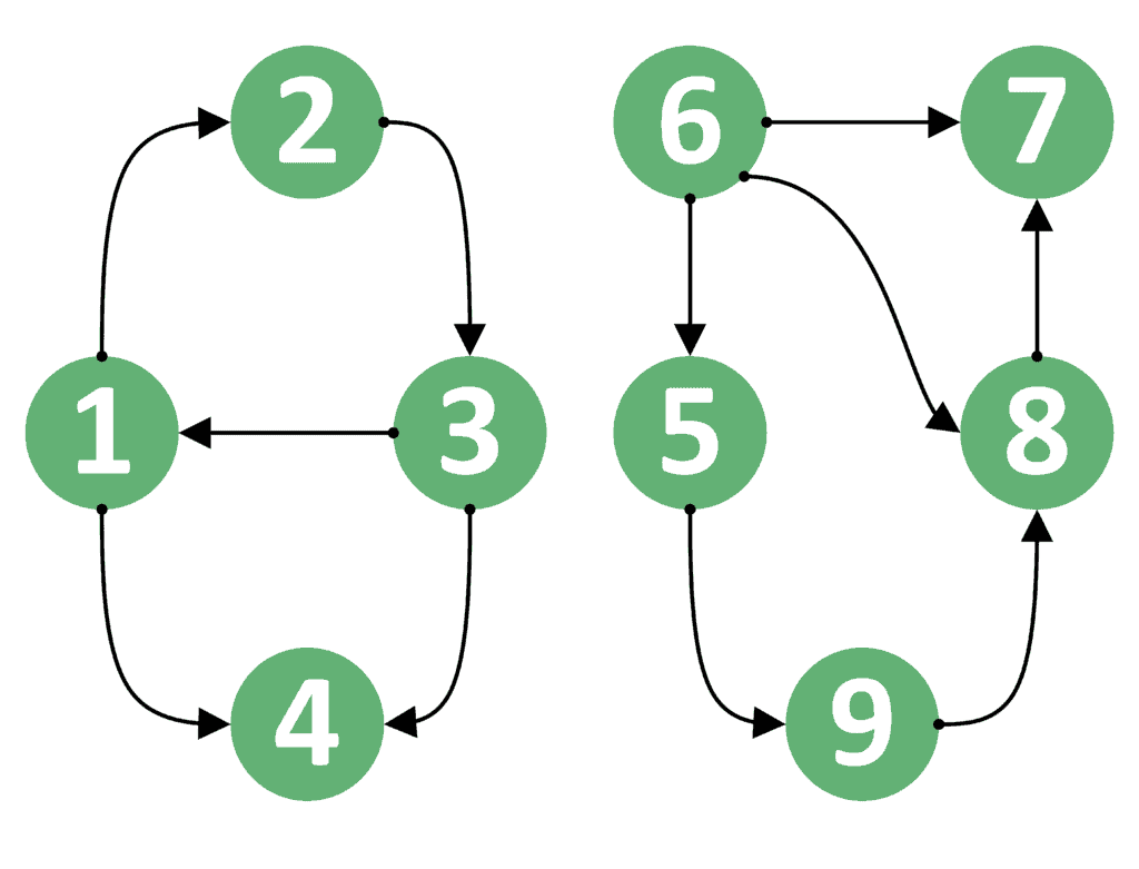
For example, suppose the starting node $u$ is node 1, and the ending node $v$ is node 3. In this case, the answer should be $true$ , because we can go from node 1 to 3 by following the path {1, 2, 3}.

Now let’s take the reversed case. If the starting node $u$ is node 3, and the ending node $v$ is node 1, the answer would still be $true$ , because we have an edge directly from node 3 to node 1.

However, this is not always the case. Suppose $u$ is node 1 and $v$ is 4. In this case, the answer is $true$ because we can go from node 1 to node 4. On the other hand, the reversed case, where $u$ is node 4, and $v$ is node 1, has the answer $false$ , because we can’t go from node 4 to node 1.

Even more, both cases for nodes 1 and 8 have an answer equal to $false$ . The reason is that we can’t go from node 1 to node 8 nor from node 8 to node 1.

From this example, we can conclude that the order of the starting and ending nodes is important. Therefore, we can’t switch nodes $u$ and $v$ in the query and expect to get the same answer.

2.2. Undirected Graphs

In undirected graphs, the situation is different. We’ll take the same example as the one provided in directed graphs, but make all edges undirected. Let’s see how will the graph look:

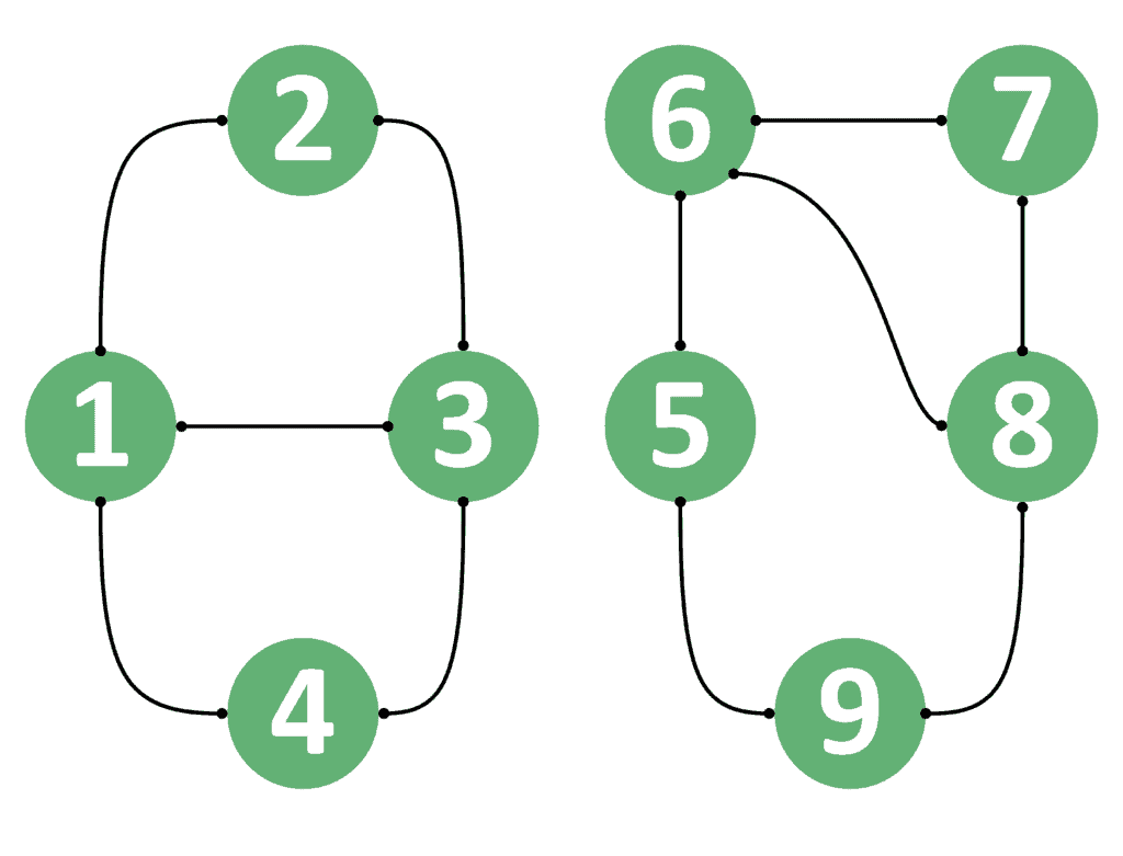
We’ll take the similar examples provided in section 2.1. Suppose $u$ is node 1 and $v$ is node 3, then the answer is $true$ because we can go from node 1 to node 3.

Similarly, we can go from node 3 to node 1 as well. Therefore, if $u$ is node 3 and $v$ is node 1, the answer will still be $true$ .

However, if we take node 1 to be $u$ and node 8 to be $v$ , the answer is $false$ because we can’t reach node 8 starting from node 1. Likewise, if $u$ is node 8 and $v$ is node 1, the answer is still $false$ .

As a result, we can conclude that if the undirected graph contains a path from one node to the other, it surely means that it contains a path from the second node to the first. The reason is that all edges are undirected and the path can be traversed in both directions.

Now that we defined our problem well enough, we can jump into discussing the solutions. We’ll assume that the graph is stored in an adjacency list for simplicity.

3. Naive Approach

The naive approach is based on performing a DFS traversal from the starting node of each query. If we manage to reach the ending node, then the answer is $true$ .

Otherwise, the answer is $false$ . Let’s take a look at the implementation of the naive approach:

algorithm NaiveApproach(G, u, v):
    // INPUT
    //     G = the Graph stored in an adjacency list
    //     u = the starting node
    //     v = the ending node
    // OUTPUT
    //     true if v can be reached starting from u, or false otherwise

    visited <- map(u : false | u in G) 
    
    return DFS(G, u, v, visited)

function DFS(G, u, v, visited):
    if u = v:
        return true
    if visited[u] = true:
        return false

    visited[u] <- true
    for next in G[u]:
        canReachV <- DFS(G, next, v, visited)
        if canReachV = true:
            return true
    
    return false

In the beginning, we’ll initialize the $visited$ array with $false$ values and call the DFS function starting from node $u$ . We’ll also pass the graph $G$ , the ending node $v$ , and the $visited$ array.

Inside the DFS function, we’ll first check whether we’ve reached the ending node $v$ . If so, then we return $true$ .

In case we haven’t reached the ending node yet, we check to see whether the current node has been visited before. If it’s been visited before, then we return $false$ , indicating that the current node was visited before. Thus, if we were able to reach $v$ , we’d have returned $true$ before.

Otherwise, we mark the current node as visited, and iterate over its neighboring nodes. For each neighbor, we perform a recursive DFS call. When performing the recursive DFS call, we pass the neighbor $next$ as the current node $u$ . This means to continue searching for $v$ starting from the node $next$ .

If this call returns $true$ , we immediately return $true$ as well, without checking other neighbors.

However, we may perform a DFS operation from all neighbors, and none of them return $true$ . In this case, we return $false$ as well, indicating that we weren’t able to reach $v$ from the current node.

The complexity of the naive approach is $O(n+m)$ for each query, where $n$ is the number of nodes, and $m$ is the number of edges inside the graph. The complexity is equal to performing a depth-first-search over a graph.

4. Finding the Component of Each Node

Let’s explain the general idea of this approach first. Then, we can discuss the implementation.

4.1. General Idea

When dealing with undirected graphs, we can come up with a better approach. The main idea is that in undirected graphs, if we can reach $v$ starting from $u$ , then we can reach $u$ starting from $v$ . The reason is that all edges can be passed in both directions.

Therefore, the only case when we can’t reach $v$ starting from $u$ is when each of them is in a different component. However, if both nodes are inside the same component, then they can be reached from one another.

Let’s divide the graph example taken in section 2.2 into two components:

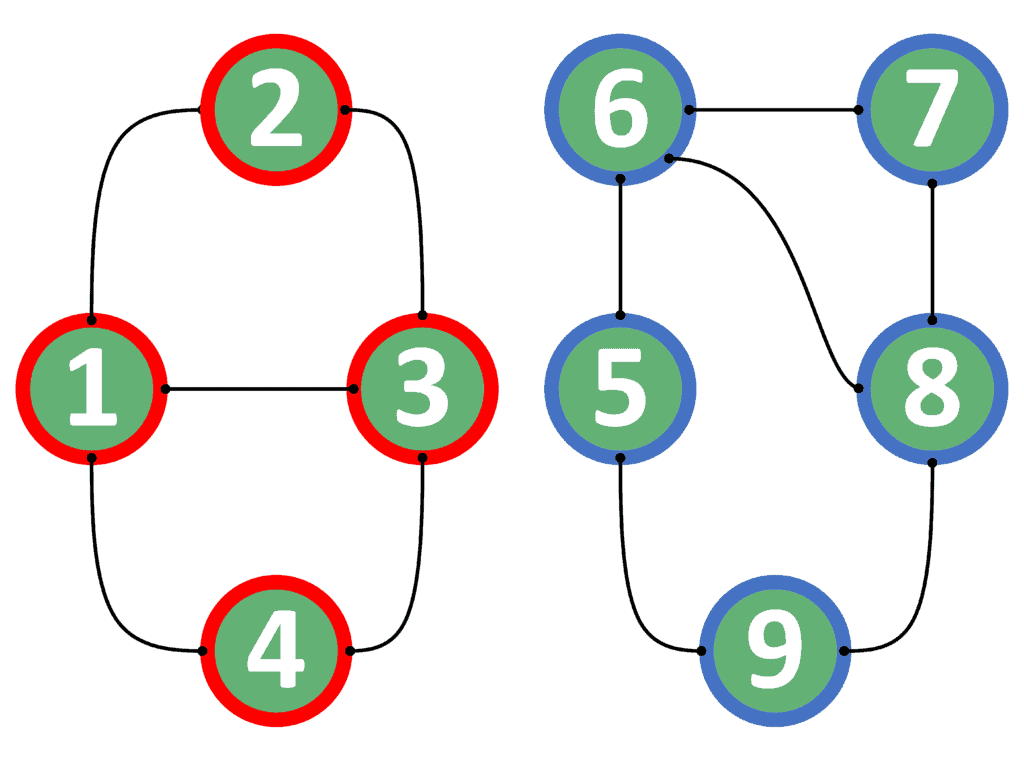
We colored each connected component with a different color. All nodes in the red component are reachable from one another. The same holds for the nodes in the blue component as well.

As a result, we can build our approach based on two steps:

Before answering any query, perform a DFS operation to divide the graph into components. In this step, we’ll assign a different component identifier for each component. Also, we’ll store the $componentId$ of each node.
For each query, check to see if nodes $u$ and $v$ are inside the same component. If so, then return $true$ . Otherwise, return $false$ .

Now, we can dive into the implementation of this approach.

4.2. Precalculation

Take a look at the implementation of the precalculation step:

algorithm PrecalculationStep(G, n):
    // INPUT
    //     G = the graph stored in an adjacency list
    //     n = the number of nodes inside the graph G
    // OUTPUT
    //     Returns the componentID array, which contains the component id of each node

    visited <- { set of visited nodes }
    componentID <- map(node : -1 | node in G)
    currentComponentID <- 0
    
    for u <- 1 to n:
        if visited[u] = false:
            currentComponentID <- currentComponentID + 1
            DFS(G, u, visited, componentID, currentComponentID)

    return componentID

function DFS(G, u, visited, componentID, currentComponentID):
    if visited[u] = true:
        return

    visited[u] <- true
    componentID[u] <- currentComponentID
    
    for next in G[u]:
        DFS(G, next, visited, componentID, currentComponentID)

We start by initializing the $visited$ array with $false$ values, the $componentID$ array with -1, and the variable $currentComponentID$ with zero.

Next, we iterate over all nodes inside the graph. For each node, if it hasn’t been visited so far, we start a DFS operation from this node. Before that, we increase the $currentComponentID$ variable by one, indicating a new component to be explored. Also, we pass several parameters to the DFS function:

The graph $G$ .
The node $u$ from which we’ll start exploring the component.
The $visited$ array, which stores which nodes have been visited so far.
The $componentID$ array, which stores the component identifier for each of the nodes explored so far.
The $currentComponentID$ variable, which contains the identifier of the current explored component.

Finally, we return the $componentID$ array.

At the beginning of the DFS function, we check to see if this node has been visited before. If so, we simply return and don’t explore the current node. Otherwise, we mark the current node as visited.

After that, we store the current component ID for the current node inside the $componentID$ array.

Finally, we iterate over all neighbors of the current node and perform a recursive DFS call starting from each of these neighbors.

The complexity of the precalculation step is $O(n+m)$ , where $n$ is the number of nodes, and $m$ is the number of edges inside the graph. Note that this step is performed only once, before answering any query.

4.3. Answering Queries

After performing the precalculation step, we can answer each query efficiently. Take a look at the implementation of answering each query:

algorithm AnswerQueries(u, v, componentID):
    // INPUT
    //     u = the starting node
    //     v = the ending node
    //     componentID = The component ID for each node
    // OUTPUT
    //     true if v can be reached starting from u, or false otherwise

    if componentID[u] = componentID[v]:
        return true
    else:
        return false

The implementation is rather simple. We just check to see if the component identifier of the node $u$ equals the component identifier of the node $v$ . If so, we return $true$ . Otherwise, we return $false$ .

The complexity of this approach is $O(1)$ because we’re only checking the values stored inside the $componentID$ array.

5. Comparison

Let’s consider the following table that lists a comparison between both approaches:

When considering undirected graphs, the approach based on connected components has a better complexity. The reason is that we perform the precalculation step only once. After that, each query can be efficiently answered in $O(1)$ .

However, we can’t use the approach based on connected components for directed graphs. Thus, we need to use the naive approach in the case of directed graphs.

6. Conclusion

In this tutorial, we presented the problem of finding whether two nodes inside a graph are connected or not.

In the beginning, we explained the problem in the case of directed and undirected graphs.

After that, we presented two approaches that can solve the problem.

Finally, we listed a comparison table that showed the main differences between both approaches and showed when to use each approach.

Full Archive

About Baeldung

Core Concepts

Operating Systems

Artificial Intelligence

Graph Theory

Latex