Calculating the Average of a Set of Circular Data

1. Introduction

In this article, we’ll study how to calculate the average of a set of circular data points. We’ll begin by defining what circular data points are and what their average would look like. Then, we’ll discuss approaches to compute average points in a set of circular data.

At the end of this tutorial, we’ll be able to implement an algorithm that calculates the average in a set of circular data points.

2. Circular Data

This tutorial will prove useful if we’re working with spatial data and building geospatial applications. Very frequently, as is the case when we work with geospatial polygons, we’re given some sets of points, and we have to find a new one that is somewhere between them. Other times, when we work with geospatial distances, we have to find a point whose sum of distances from a set of points is minimal. In these cases, we’ll want to find the average in a set of circular data points.

2.1. The Unit Circle

A set of circular data points is characterized by two coordinates: $x$ and $y$ . These coordinates must also satisfy the Pythagorean equality that $x^2 + y^2 = r^2$ for some constant radius $r$ . In the case of the unit circle, this radius is assumed to be $r=1$ :

Any other circle is a scaled-up version of this unit circle. For this reason, we can study the unit circle, knowing that any other can later be obtained by simple scaling.

2.2. Sampling the Unit Circle as a Cartesian

If we have a unit circle, we can sample a set of points from it and thus develop a set of circular points. Let’s see how we can do that and develop our dataset.

To sample a unit circle and create a dataset containing one point, we’re free to choose the first coordinate but not the second. That is to say, if we randomly pick the first coordinate, the second coordinate can’t be any arbitrary coordinate: it can only have one of two values that satisfy the Pythagorean condition we set earlier.

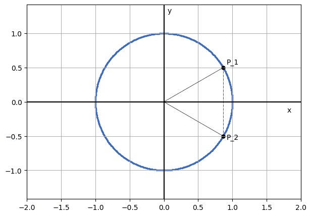
Does this mean that the second coordinate is uniquely identified? No, unfortunately, it doesn’t; for each given value of one coordinate of a point on the unit circle, there are, in fact, two possible coordinates that correspond to points in the same unit circle:

We can say, therefore, that the function that associates a $y$ coordinate to a given $x$ coordinate of a point on a circle isn’t a function but rather a map. Two points correspond to each value that we associate to a given coordinate, so a map that gives us points $(x,y)$ given an input coordinate $x$ outputs two values $y_1, y_2$ is:

$y_1, y_2 = f(x) = \begin{cases} y_1 = +\sqrt{1-x^2} \\ y_2 = -\sqrt{1-x^2} \\ \end{cases}$

If we want to generate a single point, we could randomly select an $x \in [-1, 1]$ , then flip a coin and choose $y_1$ if the coin lands on the head or $y_2$ otherwise. The point we sampled corresponds to $(x, y_1)$ in the first case or $(x, y_2)$ in the second.

If we then want to generate $\boldsymbol{n}$ points drawn from the unit circle, we could simply repeat this operation $n$ times and thus create our dataset.

If we want to create a dataset comprising points sampled randomly from the unit circle, we can’t simply accept both $(x, y_1)$ and $(x, y_2)$ for each draw and insert both into our dataset. We’d like to do that, as it would decrease the number of draws we have to perform from $n$ to $n/2$ ; however, if we did that, the points we’d draw are no longer independent draws. In fact, we’d be able to guess another point in a dataset, given a point $(x, y_1)$ , by simply flipping the sign of $y_1$ .

2.3. In Polar Coordinates

The previous method is thus not optimal since it requires drawing two random numbers per point: one for the $x$ coordinate and one for the sign of the $y$ coordinate. However, there is a better method based on a different definition of a circle.

A unit circle can be defined as the space spanned by a rotating segment of length 1 around the origin:

With this type of definition, a point on this circle can be uniquely identified by determining the angle existing between the rotating segment and one of the two basis vectors for the plane:

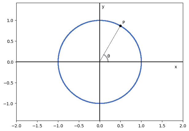
Most frequently, we select the $x$ axis as the one with respect to which we measure the angle. If the points come in polar coordinates, then they are defined as an ordered pair $(r, \theta)$ , where $r$ is a radius, and $\theta$ is the angle with the $x$ axis. If we have a point in polar coordinates, but we want it in Cartesian coordinates, we can always convert via this transformation:

$\begin{cases} x = r \cos(\theta) \\ y = r \sin(\theta) \end{cases}$

Notice that, for the unit circle, the Cartesian coordinates of a point equal the output of the two trigonometric functions associated with the corresponding angle.

If we’re working in polar coordinates, and we want to draw a random point on a circle of radius $r$ , all we have to do is draw a random angle $\theta$ from the uniform distribution $[0, 360)$ , and repeat for as often as necessary.

3. Calculating the Average of a Set of Circular Data

3.1. The Average of a Set

Now that we have a method for drawing random points from a circle, we can calculate their average. In general, if we have a set $X$ of $n\in\mathbb{N}, n \geq 1$ elements drawn from $\mathbb{R}$ , such that $X = \{x_1, x_2, ..., x_n\}$ , then we define its average $\text{Avg}(X)$ as:

$\text{Avg}(X) = \frac{\sum_{i=1}^{n} x_i}{n}$

The average of $X$ is provably contained in $\mathbb{R}$ . This is because the set from which the variable is created, the set of the real numbers, is closed under the operations of addition and division that make up $\text{Avg}(X)$ .

3.2. The Average in a Bivariate Distribution

If we have a bivariate distribution $(X,Y)$ of $n$ real numbers, such that $X = \{x_1, x_2, ..., x_n\}$ and $Y = \{y_1, y_2, ..., y_n\}$ , we can define the average $\text{Avg}(X,Y)$ of this bivariate distribution as:

$\text{Avg}(X,Y) = (\frac{\sum_{i=1}^{n} x_i}{n}, \frac{\sum_{i=1}^{n} y_i}{n})$

In other words, if we have two real variables, the average of the bivariate distribution can be calculated by independently computing the average of each of the two variables. The same principle generalizes to any $k$ -variate distribution comprising $k$ independent variables. In that case, we simply compute the average of each independent variable and consider, as the average for the multivariate distribution, the tuple comprising each computed average.

3.3. Average of a Set of Circular Data

A set of points drawn from a circle doesn’t however comprise independent variables, and it doesn’t, therefore, fall under the hypothesis of multivariate distribution described above. This is because we impose an additional constraint between the $k$ coordinates of the points of a circle. In fact, if the point $P = (p_1, p_2, ..., p_k)$ is on a $k$ -sphere, then the following relationship must persist:

$p_1^2 + p_2^2 + ... + p_k^2 = r^2$

There is however no guarantee that the average of the coordinates of several points, with each point satisfying the previous condition for the same, unique $r$ , also satisfies that same condition.

Let’s consider the trivial case in which the two points, $P_1 = (1,0)$ and $P_2 = (-1,0)$ , lie at two opposite poles of the unit circle: both points then satisfy the conditions that they lie on a circle of radius $r=1$ . The average computed according to the previous rule, as $\text{Avg}(X,Y)$ , is however:

$\text{Avg}(X,Y) = \frac{1+(-1)}{2}, \frac{0+0}{2} = (0,0)$

This average doesn’t satisfy the condition of the unit circle because its squared coordinates aren’t equal to 1. This may satisfy us in some cases, as we might, for example, be interested in finding the barycenter for a gravitational system of static objects of equal mass. In that case, the average computed above will suffice.

However, if we want to compute averages that lie on the same circle as the points they refer to, we need to impose some additional constraints.

3.4. The Average Itself Is on a Circle

To find an average of points that lie on a circle, with the average itself on that circle, we should refer to the considerations we made above and convert all coordinates to their polar form. Then, we compute the average of the polar coordinates, which guarantees that the result lies on the circle.

If we want the average of the two points $P_1 = (1,0)$ and $P_2 = (-1,0)$ , in this order, to be located at $(0,1)$ , we could then calculate a value of $\theta_1 = 0$ to $P_1$ and $\theta_2 = 180$ to $P_2$ . In doing so, we can find the average angle $\overline{\theta}$ as:

$\overline{\theta} = \frac{\theta_1 + \theta_2} {2} = \frac{0 + 180} {2} = 90$

This gives us a nice angle of 90 degrees, orthogonal to the $x$ axis, as we’d expect.

4. The Algorithm to Compute the Average

4.1. Transforming Into Polar Coordinates

In general terms, the procedure for computing the average of a set of circular data is as follows.

We begin with a set of $n$ points $\{P_1, P_2, ..., P_n\}$ . We can express their coordinates as tuples, as $\{(x_1, y_1), (x_2, y_2), ..., (x_n, y_n)\}$ . Then, if we assume that they all belong to the same circle, we compute the circle’s radius as $r = \sqrt{x_1^2 + y_1^2}$ . We only need to do it for the first tuple since the radius is constant.

In polar form, the radius $r$ is the first of the two coordinates for each of the $n$ points. The remaining coordinate, the angle $\boldsymbol{\theta}$ , can be calculated as a function of a temporary variable $\theta^\prime$ . We construct $\theta^\prime$ as:

$\theta^\prime = 2 \arctan \frac{y}{x+r}$

Then, according to the signs of $x$ and $y$ , we generate $\theta$ from $\theta^\prime$ as:

$\begin{cases} \theta = \theta^\prime & x \geq 0 \wedge y \geq 0 \\ \theta = \pi - \theta^\prime & x < 0 \wedge y \geq 0 \\ \theta = \pi + \theta^\prime & x < 0 \wedge y < 0 \\ \theta = 2\pi - \theta^\prime & x \geq 0 \wedge y < 0 \\ \end{cases}$

4.2. Averaging the Angle

Once the set ${\theta_1, \theta_2, ..., \theta_n}$ has thus been computed, its average can be calculated as:

$\text{Avg}(\theta) = \frac {\sum_{i=1}^{n} \theta_i} {n}$

The point on the circle that corresponds to $(r, \text{Avg}(\theta))$ is therefore the one that we find by transforming back into Cartesian coordinates:

$\begin{cases} \overline{x} = r \cos(\text{Avg}(\theta)) \\ \overline{y} = r \sin(\text{Avg}(\theta)) \end{cases}$

This point with coordinates $(\overline{x}, \overline{y})$ is, finally, the average of the points of the set of circular data. We can prove that this point is guaranteed to lie on the circle with radius $r$ :

$\begin{matrix} \overline{x}^2 + \overline{y}^2 = r^2 & \text{substitute on the LHS} \\ (r \cos(\text{Avg}(\theta))^2 + (r \sin(\text{Avg}(\theta))^2 = r^2 & \text{collect }r^2\text{ on the LHS} \\ r^2 \cdot (\cos^2(\text{Avg}(\theta)) + \sin^2(\text{Avg}(\theta))) & \text{use the trigonometric identity } \cos^2 (\alpha) + \sin^2(\alpha) = 1 \\ r^2 \cdot (1) = r^2 & \text{Q.E.D.} \end{matrix}$

The average point $\overline{P}$ is thus $\overline{P} = (\overline{x},\overline{y})$ .

4.3. If the Radius Isn’t Constant

The last case to consider is where the radius can vary. This can happen if all points are drawn from a spheroid with the same center but with some variance in its radius. This is the case, for example, for all points drawn from the surface of Earth since the radius of the planet isn’t constant.

In this case, it isn’t sufficient to average out the angles $\theta_i$ . Instead, we have to average two variables: the angle itself, and the radius as well, with the latter calculated with respect to every single point.

For each point $P = (x_i, y_i)$ , we can obtain the associated radius $r_i$ as $r_i = \sqrt{x^2+y^2}$ . Then, the average point $\overline{P}$ for the set of points becomes $\overline{P} = (\text{Avg}(r), \text{Avg}(\theta))$ , found by averaging out all computed radii.

5. Conclusions

In this article, we studied how to calculate the average of a set of circular data. We began by defining the conditions that make a set of points circular. We also studied how to create a set of circular points by randomly drawing from a circle.

Then, we defined the concept of average in relation to a set of points. Finally, we also added the additional constraint that the average, itself, must be a point on a circle and relaxed the constraint that the radius is constant among all points.

Full Archive

About Baeldung

Core Concepts

Operating Systems

Artificial Intelligence

Graph Theory

Latex