

Yes, we're now running our only Summer Sale. All Courses are 30% off until 20th July, 2026:
Learn through the super-clean Baeldung Pro experience:
>> Membership and Baeldung Pro.
No ads, dark-mode and 6 months free of IntelliJ Idea Ultimate to start with.
1. Introduction
The idea of augmenting paths comes up in two different contexts in computer science. These are matching theory and the maximum flow problem. In both cases, we can use augmenting paths to increase the size of an existing solution. This way, the solution gets closer to being optimal.
In this tutorial, we’ll discuss what exactly are augmenting paths. First, we’ll see them in the context of matchings in a graph. Then, we’ll study them in relation to the maximum flow problem. We’ll also briefly discuss some algorithms that make use of augmenting paths.
2. Augmenting Paths in Matching Theory
2.1. Definitions
Before we can talk about what augmenting paths are with respect to matchings, we need a few definitions. A matching  is a subset of the edges of a graph
  such that no two edges in share a common vertex.
If has the largest size amongst all matchings in  , then we call a maximum matching. We call a vertex of matched by if touches that vertex. Otherwise, the vertex is unmatched.
On the left below is an example of a matching in a bipartite graph (the red-colored edges represent a matching):
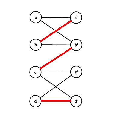
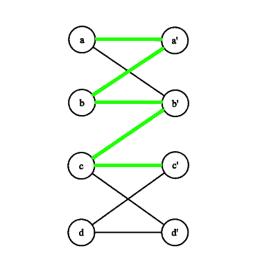
A path in which starts at an unmatched vertex and then contains, alternately, edges from  and , is an alternating path with respect to . We call an alternating path that ends in an unmatched vertex an augmenting path.
For the matching above, the path  is an example of both an alternating path and an augmenting path. This path is highlighted in green on the right.
2.2. How Are Augmenting Paths Used for Finding Maximum Matchings?
We can use an augmenting path  to turn a matching into a larger matching by taking the symmetric difference of with the edges of . In other words, we remove edges from which are in both and . We add/keep all other edges. We can best illustrate this by an example:
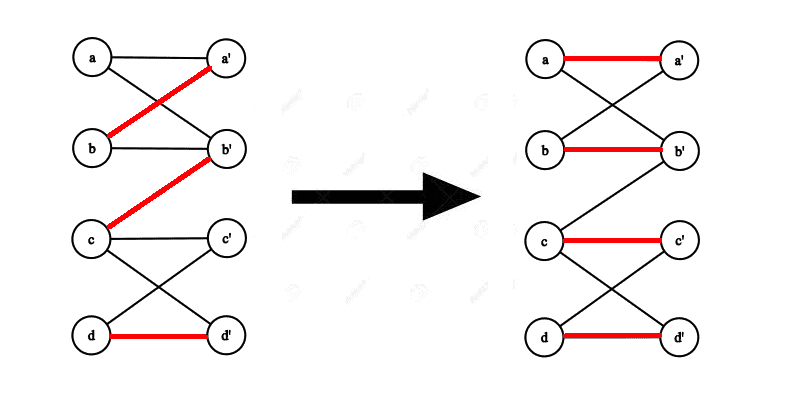
The augmenting path we used is shown below:
Here we used the augmenting path (shown in green) to augment the initial matching to obtain a bigger matching  . The edges
  and
and  were removed from and the edges
  ,
,  , and
, and  were added to . We also kept the edge
  in .
in .
We can prove that if we start with any matching and repeatedly augment it by augmenting paths, we’ll always eventually obtain matching of optimal size, i.e., a maximum matching.
This is the key intuition behind any algorithm for finding maximum matchings.
2.3. Algorithms That Use Augmenting Paths to Find Maximum Matchings
Two examples of famous algorithms that use augmenting paths are the Hungarian Algorithm and the Blossom Algorithm. We can use the former to find maximum matchings in a bipartite graph and the latter to find maximum matchings in a general graph. To find an augmenting path, algorithms will typically use a tree search such as depth-first search or breadth-first search, with some minor modifications/additions.
3. Augmenting Paths in the Maximum Flow Problem
3.1. Some Initial Definitions
Let’s look at a few key definitions first. Then we’ll see what an augmenting path is in the maximum flow problem.
A flow network is a directed graph in which each edge  has a nonnegative capacity
  . We don’t allow self-loops and
  if the edge doesn’t exist. Finally, if there exists an edge in the network then the reverse edge
  doesn’t exist.
Here is an example of a flow network which contains a flow with a total value of 19:
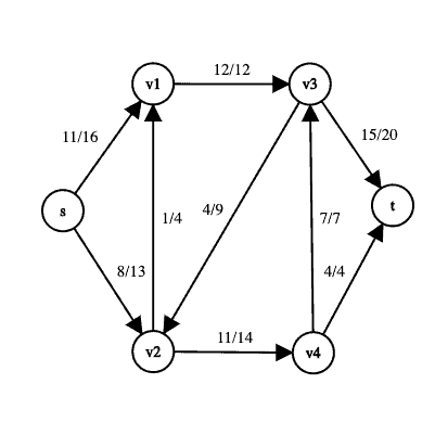
The edge labels take the form  to communicate the fact that an edge has a capacity of
  and a flow of
  .
.
There are two special vertices in a flow network; the source  and the sink
  . The source can be thought of as a vertex that produces some material, and the sink is a vertex that consumes the material.
We define a flow in a flow network as an assignment of nonnegative real-numbers to the edges of the network such that the values do not exceed the capacity constraints and the principle of flow conservation holds. Flow conservation says that at every node except the source and the sink, the total incoming flow must equal the total outgoing flow.
The total value of a flow , denoted by  , is defined as the total flow leaving the source minus the total flow coming into the source. In the maximum-flow problem, we’re given a flow network , and we want to find a flow of maximum value.
3.2. Residual Networks
Given a flow network , the corresponding residual network  represents how we can change the flow on different edges of . For an edge in with flow less than that edge’s capacity, there will be a corresponding edge in that has a residual capacity of the original edge’s capacity minus the flow on that edge.
If an edge in the original graph is saturated (its flow equals its capacity), then the corresponding edge is omitted from the residual graph as it cannot admit anymore flow.
We can also have edges in the residual graph that are not in the original graph. These are edges that allow an algorithm to send flow back on an edge, thereby reducing the original flow on that edge. If we have an edge in with a certain amount of flow on it, then we’ll have an opposite edge in the residual graph with a capacity equal to that flow.
Below is an example of the residual graph for the flow network shown above:
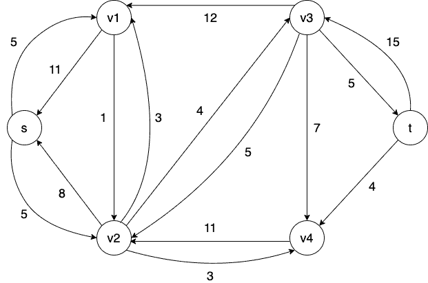
If we look at this residual network, we can see the above concepts in action.
For example, we can see that there is an edge in with a capacity 16 from to  with a flow amount of 11 units. Therefore, we have two corresponding edges in . One edge is a forward edge from to with a residual capacity of 5. The other is a back edge from to with a residual capacity 11.
The forward edge represents the fact that we can still send an additional 5 units of flow from to . The back edge communicates that we can send 11 units of flow back from to (which is the same as reducing the flow going from to ).
3.3. Augmenting Paths
Now that we have defined what a residual network is, we can talk about augmenting paths. Given a flow network , an augmenting path is a simple path from the source to the sink in the corresponding residual network . Intuitively, an augmenting path tells us how we can change the flow on certain edges in so that we increase the overall flow from the source to the sink.
For example, here is an augmenting path (shaded in red) in the previous residual graph:
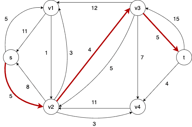
If we treat this network as a flow network, we can think of sending 4 units of flow along this path from to . Sending flow along this path in corresponds to increasing and decreasing the flow on particular edges in . In this case, we can send at most 4 units of flow along the augmenting path in so that in , we increase the flow by 4 units on edges  and
and  , and decrease the flow by 4 units on the edge
  .
.
This brings up an important point related to augmenting paths. Although an augmenting path increases the overall flow, it can not only increase the flow on an edge; it can also decrease it. It can be easy to think that since an augmenting path augments the flow, it’s only increasing edge flows. But this is not necessarily true.
We can prove that given any flow in a flow network and an augmenting path in , augmenting with this path will give us a new flow in with a higher value.
3.4. Algorithms That Use Augmenting Paths to Find the Maximum Flow
Perhaps the most well-known algorithm which uses augmenting paths to find a maximum flow is the Ford-Fulkerson algorithm. The intuition behind the Ford-Fulkerson method is simple: while there exists an augmenting path with respect to the current flow in the network, augment that flow using the augmenting path to obtain a new flow. This strategy guarantees that we’ll find a maximum flow because of a famous theorem called the max-flow min-cut theorem, which tells us that a flow has maximum value if and only if there is no augmenting path in its residual graph.
Based on how we find augmenting paths in the Ford-Fulkerson method, we can obtain better running times. For example, we can choose the shortest path with available capacity as our augmenting path in each iteration. Then we’ll get a faster implementation of Ford-Fulkerson. This is called the Edmonds-Karp Algorithm.
Another algorithm for computing maximum flows is called Dinic’s Algorithm. Instead of simply finding one augmenting path in each iteration, it makes use of two important ideas: the level graph and the blocking flow. By finding a blocking flow, Dinic’s algorithm computes all augmenting paths of a particular length. Then it uses this blocking flow to augment the flow.
4. Conclusion
In this article, we have studied what augmenting paths are in the contexts of maximum matchings and maximum flows. We have also briefly discussed some algorithms which make use of augmenting paths.