

Learn through the super-clean Baeldung Pro experience:
>> Membership and Baeldung Pro.
No ads, dark-mode and 6 months free of IntelliJ Idea Ultimate to start with.
Last updated: May 23, 2025
Learn through the super-clean Baeldung Pro experience:
>> Membership and Baeldung Pro.
No ads, dark-mode and 6 months free of IntelliJ Idea Ultimate to start with.
In this tutorial, we’ll study the ACF and PACF plots of ARMA-type models to understand how to choose the best  and
and  values from them.
We’ll start our discussion with some base concepts such as ACF plots, PACF plots, and stationarity. After that, we’ll explain the ARMA models as well as how to select the best and from them. Lastly, we’ll propose a way of solving this problem using data science and the machine learning approach.
The autocorrelation function (ACF) is a statistical technique that we can use to identify how correlated the values in a time series are with each other. The ACF plots the correlation coefficient against the lag, which is measured in terms of a number of periods or units. A lag corresponds to a certain point in time after which we observe the first value in the time series.
The correlation coefficient can range from -1 (a perfect negative relationship) to +1 (a perfect positive relationship). A coefficient of 0 means that there is no relationship between the variables. Also, most often, it is measured either by Pearson’s correlation coefficient or by Spearman’s rank correlation coefficient.
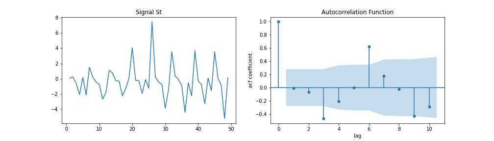
It’s most often used to analyze sequences of numbers from random processes, such as economic or scientific measurements. It can also be used to detect systematic patterns in correlated data sets such as securities prices or climate measurements. Usually, we can calculate the ACF using statistical packages from Python and R or using software such as Excel and SPSS. Below, we can see an example of the ACF plot:
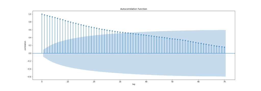
Blue bars on an ACF plot above are the error bands, and anything within these bars is not statistically significant. It means that correlation values outside of this area are very likely a correlation and not a statistical fluke. The confidence interval is set to 95% by default.
Notice that for a lag zero, ACF is always equal to one, which makes sense because the signal is always perfectly correlated with itself.
To summarize, autocorrelation is the correlation between a time series (signal) and a delayed version of itself, while the ACF plots the correlation coefficient against the lag, and it’s a visual representation of autocorrelation.
Partial autocorrelation is a statistical measure that captures the correlation between two variables after controlling for the effects of other variables. For example, if we’re regressing a signal  at lag
  (
( ) with the same signal at lags
  ,
,  and
and  (
( ,
,  ,
,  ), the partial correlation between and is the amount of correlation between and that isn’t explained by their mutual correlations with and .
That being said, the way of finding PACF between and is to use regression model
(1) 
where  ,
,  and
and  are coefficients and
  is error. From the regression formula above, the PACF value between and is the coefficient
  . This coefficient will give us direct effect of time-series to the time-series because the effects of and are already captured by and .
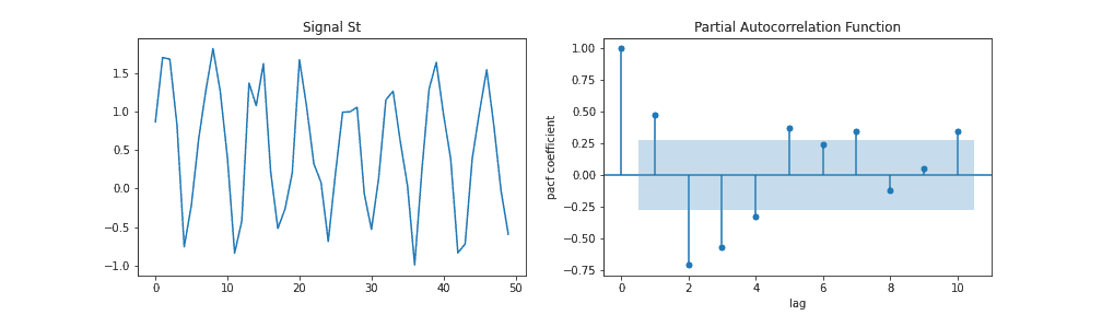
The figure below presents the PACF plot:
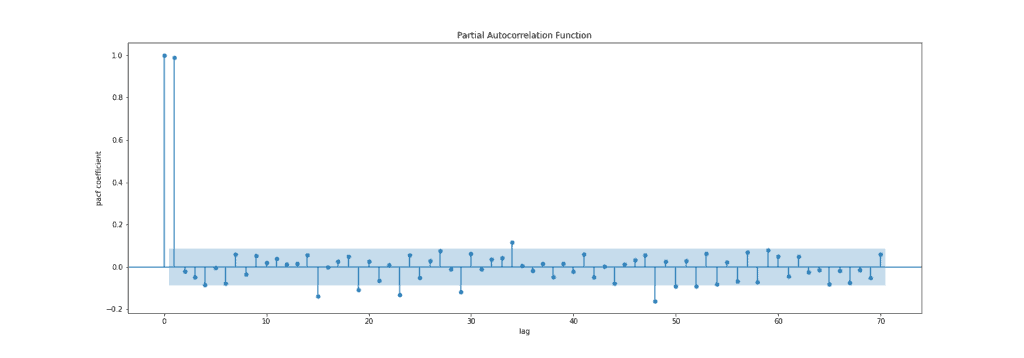
To summarize, a partial autocorrelation function captures a “direct” correlation between time series and a lagged version of itself.
When it comes to time series forecasting, the stationarity of a time series is one of the most important conditions that the majority of algorithms require. Briefly, time-series is stationary (weak stationarity) if these conditions are met:
has a constant mean. has a constant standard deviation.. If has a repeating pattern within a year, then it has seasonality.We can check the stationarity of the signal visually (approximation) or using some statistical hypothesis for a more precise answer. For that purpose, we can mention two tests:
If signal is non-stationary, we can convert them into stationary signal  by differencing
(2) 
or calculating percent of change
(3) 
Notwithstanding these transformations, signal won’t always be stationary. It is rare but can happen. In that case, if stays non-stationary, we can apply the same transformation to signal .
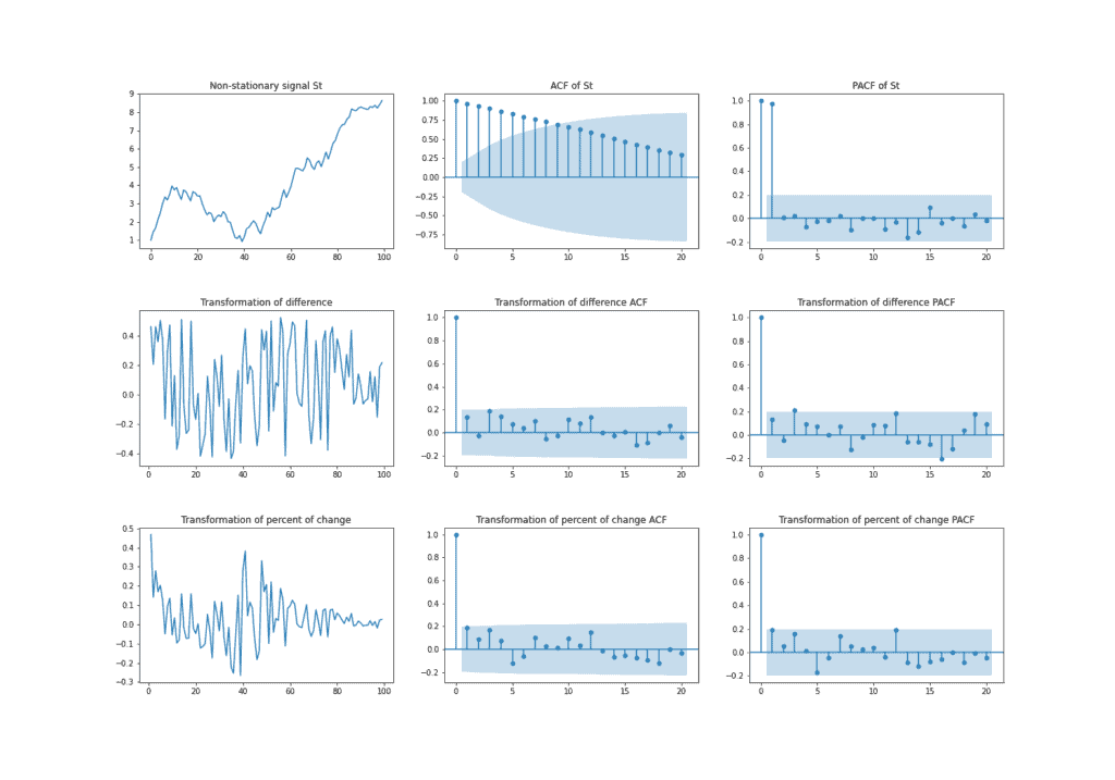
The example below shows the non-stationary time series followed by the two transformations mentioned above. Also, we can see how AFC and PACF change as the signal goes through transformations. Because of the positive trend, signal has a high correlation with a lagged version of itself, and thus ACF plot shows a slow decrease. In opposite, for the two presented transformations, AFC only has a significant correlation at lag zero.
The ARMA( ) model is a time series forecasting technique used in economics, statistics, and signal processing to characterize relationships between variables. This model can predict future values based on past values and has two parameters, and , which respectively define the order of the autoregressive part (AR) and moving average part (MA).
We’ll define both parts of the ARMA model separately in order to easier understand them.
But before that, we need to know that both AR and MA models require the stationarity of the signal. Usually, using non-stationary time series in regression models can lead to a high R-squared value and statistically significant regression coefficients. These results are very likely misleading or spurious.
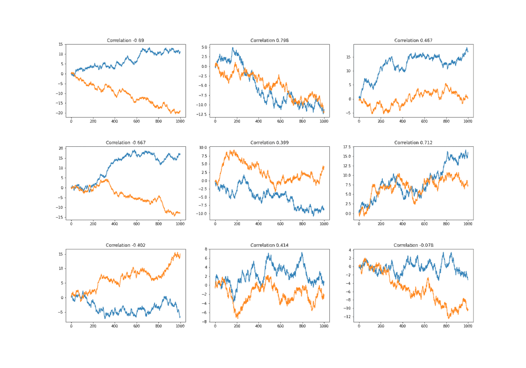
It’s because there is probably no real relationship between them and the only common thing is that they’re growing (declining) over time. We can test that by computing the correlation between two random walks defined by the formula
(4) ![\begin{align*} y_{t} = y_{t-1} + \epsilon_{t}, \epsilon_{t} \in [-1, 1]. \end{align*}](/wp-content/ql-cache/quicklatex.com-50ac4a97259797945fe4c243bf112369_l3.svg "Rendered by QuickLaTeX.com")
In the figure below, we generated nine pairs of random walks. As a result, we can see that most of the pairs have a high correlation that is obviously spurious.
The autoregressive model is a statistical model that expresses the dependence of one variable on an earlier time period. It’s a model where signal depends only on its own past values. For example, AR(3) is a model that depends on 3 of its past values and can be written as
(5) 
where  are coefficients and
  is error. We can select the order for AR() model based on significant spikes from the PACF plot. One more indication of the AR process is that the ACF plot decays more slowly.
For instance, we can conclude from the example below that the PACF plot has significant spikes at lags 2 and 3 because of the significant PACF value. In contrast, for everything within the blue band, we don’t have evidence that it’s different from zero. Also, we could try for other values of lag that are outside of the blue belt. To conclude, everything outside the blue boundary of the PACF plot tell us the order of the AR model:
The MA() model calculates its forecast value by taking a weighted average of past errors. It has the ability to capture trends and patterns in time series data. For example, MA(3) for a signal can be formulated as
(6) 
where  is the mean of a series,
  are coefficients and
  are errors that have a normal distribution with mean zero and standard deviation one (sometimes called white noise).
In contrast to the AR model, we can select the order for model MA() from ACF if this plot has a sharp cut-off after lag . One more indication of the MA process is that the PACF plot decays more slowly.
Similar to selecting for the AR model, in order to select the appropriate order for the MA model, we need to analyze all spikes higher than the blue area. In that sense, from the image below, we can try using  or
or  .
.
ARMA( ) is a combination of AR() and MA() models. For example, ARMA(3,3) of signal the can be formulated as
(7) 
where  ,
,  are coefficients and error. We’ve already described the way of choosing order and in the section for AR and MA models.
Sometimes it’s very hard and time expensive to find the right order of and for the ARMA model by analyzing ACF and PACF plots as we mentioned above. Therefore, there are some easier approaches where it comes to tuning this model. Today, most statistical tools have integrated functionality that is often called “auto ARIMA”.
For example, in python and R, the auto ARIMA method itself will generate the optimal and parameters, which would be suitable for the data set to provide better forecasting. The high-level logic behind that is the same as the logic behind hyperparameter tuning of any other machine learning model. We need to try some combinations of and parameters and compare results using a validation set.
Since our search space is not big, usually values and are not higher than 10, we can apply a popular technique for hyperparameter optimization called grid search. Grid search is simply an exhaustive search through a manually specified subset of the hyperparameter space of a learning algorithm. Basically, it means that this method will try each combination of and from the specified subset that we provided.
Also, in order to find the best combination of and , we need to have some objective function that will measure model performance on a validation set. Usually, we can use AIC and BIC for that purpose. The lower the value of these criteria, the better the model is.
6.1. Akaike Information Criteria (AIC)
AIC stands for Akaike Information Criteria, and it’s a statistical measure that we can use to compare different models for their relative quality. It measures the quality of the model in terms of its goodness-of-fit to the data, its simplicity, and how much it relies on the tuning parameters. The formula for AIC is
(8) 
where  is a log-likelihood, and
  is a number of parameters. For example, the AR() model has
  parameters. From the formula above, we can conclude that AIC prefers a higher log-likelihood that indicates how strong the model is in fitting the data and a simpler model in terms of parameters.
6.2. Bayesian Information Criteria (BIC)
In addition to AIC, the BIC (Bayesian Information Criteria) uses one more indicator  that defines the number of samples used for fitting. The formula for BIC is
(9) 
Finally, since we’re dealing with time series, we would need to utilize appropriate validation techniques for parameter tuning. This is important because we want to simulate the real-time behavior of the data flow. For instance, it wouldn’t be correct to use a data sample  to predict data sample
  if comes before by time because in real life we can’t use information from the future to predict data in real-time.
Thus, one popular validation technique used for tuning time-series-based machine learning models is cross-validation for time-series. The goal is to see which hyperparameters of the model give the best result in sense of our selected measurement metric on the training data and then use that model for future predictions.
For example, if our data consist of five time-points, we can make a train-test split as:
Of course, one time-point might not be enough as the starting training set, but instead of one, we can start with starting points and follow the same logic.
In this article, we’ve presented some important terms when it is about time-series forecasting.
Time-series forecasting is a very complicated and difficult task, and there is no one right method how to do this. In practice and from the examples of ACF and PACF above, we’ve seen that selecting the right and by analyzing only diagrams can be a fairly indeterminant task. Therefore, we presented one more way from practice for choosing the right and based on methods from machine learning.