Mocking is an essential part of unit testing, and the Mockito library makes it easy to write clean and intuitive unit tests for your Java code.
Get started with mocking and improve your application tests using our Mockito guide:
Handling concurrency in an application can be a tricky process with many potential pitfalls. A solid grasp of the fundamentals will go a long way to help minimize these issues.
Get started with understanding multi-threaded applications with our Java Concurrency guide:
Spring 5 added support for reactive programming with the Spring WebFlux module, which has been improved upon ever since. Get started with the Reactor project basics and reactive programming in Spring Boot:
Since its introduction in Java 8, the Stream API has become a staple of Java development. The basic operations like iterating, filtering, mapping sequences of elements are deceptively simple to use.
But these can also be overused and fall into some common pitfalls.
To get a better understanding on how Streams work and how to combine them with other language features, check out our guide to Java Streams:
Explore Spring Boot 3 and Spring 6 in-depth through building a full REST API with the framework:
Yes, Spring Security can be complex, from the more advanced functionality within the Core to the deep OAuth support in the framework.
I built the security material as two full courses - Core and OAuth, to get practical with these more complex scenarios. We explore when and how to use each feature and code through it on the backing project.
You can explore the course here:
Spring Data JPA is a great way to handle the complexity of JPA with the powerful simplicity of Spring Boot.
Get started with Spring Data JPA through the guided reference course:
Refactor Java code safely — and automatically — with OpenRewrite.
Refactoring big codebases by hand is slow, risky, and easy to put off. That’s where OpenRewrite comes in. The open-source framework for large-scale, automated code transformations helps teams modernize safely and consistently.
Each month, the creators and maintainers of OpenRewrite at Moderne run live, hands-on training sessions — one for newcomers and one for experienced users. You’ll see how recipes work, how to apply them across projects, and how to modernize code with confidence.
Join the next session, bring your questions, and learn how to automate the kind of work that usually eats your sprint time.
Yes, we're now running our only Summer Sale. All Courses are 30% off until 20th July, 2026:
Yes, we're now running our only Summer Sale. All Courses are 30% off until 20th July, 2026:
1. Overview
TensorFlow is an open source library for dataflow programming. This was originally developed by Google and is available for a wide array of platforms. Although TensorFlow can work on a single core, it can as easily benefit from multiple CPU, GPU or TPU available.
In this tutorial, we’ll go through the basics of TensorFlow and how to use it in Java. Please note that the TensorFlow Java API is an experimental API and hence not covered under any stability guarantee. We’ll cover later in the tutorial possible use cases for using the TensorFlow Java API.
2. Basics
TensorFlow computation basically revolves around two fundamental concepts: Graph and Session. Let’s go through them quickly to gain the background needed to go through the rest of the tutorial.
2.1. TensorFlow Graph
To begin with, let’s understand the fundamental building blocks of TensorFlow programs. Computations are represented as graphs in TensorFlow. A graph is typically a directed acyclic graph of operations and data, for example:
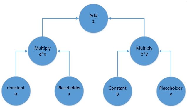
The above picture represents the computational graph for the following equation:
f(x, y) = z = a*x + b*yA TensorFlow computational graph consists of two elements:
- Tensor: These are the core unit of data in TensorFlow. They are represented as the edges in a computational graph, depicting the flow of data through the graph. A tensor can have a shape with any number of dimensions. The number of dimensions in a tensor is usually referred to as its rank. So a scalar is a rank 0 tensor, a vector is a rank 1 tensor, a matrix is a rank 2 tensor, and so on and so forth.
- Operation: These are the nodes in a computational graph. They refer to a wide variety of computation that can happen on the tensors feeding into the operation. They often result in tensors as well which emanate from the operation in a computational graph.
2.2. TensorFlow Session
Now, a TensorFlow graph is a mere schematic of the computation which actually holds no values. Such a graph must be run inside what is called a TensorFlow session for the tensors in the graph to be evaluated. The session can take a bunch of tensors to evaluate from a graph as input parameters. Then it runs backward in the graph and runs all the nodes necessary to evaluate those tensors.
With this knowledge, we are now ready to take this and apply it to the Java API!
3. Maven Setup
We’ll set-up a quick Maven project to create and run a TensorFlow graph in Java. We just need the tensorflow dependency:
<dependency>
    <groupId>org.tensorflow</groupId>
    <artifactId>tensorflow</artifactId>
    <version>1.12.0</version>
</dependency>
4. Creating the Graph
Let’s now try to build the graph we discussed in the previous section using the TensorFlow Java API. More precisely, for this tutorial we’ll be using TensorFlow Java API to solve the function represented by the following equation:
z = 3*x + 2*yThe first step is to declare and initialize a graph:
Graph graph = new Graph()Now, we have to define all the operations required. Remember, that operations in TensorFlow consume and produce zero or more tensors. Moreover, every node in the graph is an operation including constants and placeholders. This may seem counter-intuitive, but bear with it for a moment!
The class Graph has a generic function called opBuilder() to build any kind of operation on TensorFlow.
4.1. Defining Constants
To begin with, let’s define constant operations in our graph above. Note that a constant operation will need a tensor for its value:
Operation a = graph.opBuilder("Const", "a")
  .setAttr("dtype", DataType.fromClass(Double.class))
  .setAttr("value", Tensor.<Double>create(3.0, Double.class))
  .build();
Operation b = graph.opBuilder("Const", "b")
  .setAttr("dtype", DataType.fromClass(Double.class))
  .setAttr("value", Tensor.<Double>create(2.0, Double.class))
  .build();
Here, we have defined an Operation of constant type, feeding in the Tensor with Double values 2.0 and 3.0. It may seem little overwhelming to begin with but that’s just how it is in the Java API for now. These constructs are much more concise in languages like Python.
4.2. Defining Placeholders
While we need to provide values to our constants, placeholders don’t need a value at definition-time. The values to placeholders need to be supplied when the graph is run inside a session. We’ll go through that part later in the tutorial.
For now, let’s see how can we define our placeholders:
Operation x = graph.opBuilder("Placeholder", "x")
  .setAttr("dtype", DataType.fromClass(Double.class))
  .build();
Operation y = graph.opBuilder("Placeholder", "y")
  .setAttr("dtype", DataType.fromClass(Double.class))
  .build();
Note that we did not have to provide any value for our placeholders. These values will be fed as Tensors when run.
4.3. Defining Functions
Finally, we need to define the mathematical operations of our equation, namely multiplication and addition to get the result.
These are again nothing but Operations in TensorFlow and Graph.opBuilder() is handy once again:
Operation ax = graph.opBuilder("Mul", "ax")
  .addInput(a.output(0))
  .addInput(x.output(0))
  .build();
Operation by = graph.opBuilder("Mul", "by")
  .addInput(b.output(0))
  .addInput(y.output(0))
  .build();
Operation z = graph.opBuilder("Add", "z")
  .addInput(ax.output(0))
  .addInput(by.output(0))
  .build();
Here, we have defined there Operation, two for multiplying our inputs and the final one for summing up the intermediate results. Note that operations here receive tensors which are nothing but the output of our earlier operations.
Please note that we are getting the output Tensor from the Operation using index ‘0’. As we discussed earlier, an Operation can result in one or more Tensor and hence while retrieving a handle for it, we need to mention the index. Since we know that our operations are only returning one Tensor, ‘0’ works just fine!
5. Visualizing the Graph
It is difficult to keep a tab on the graph as it grows in size. This makes it important to visualize it in some way. We can always create a hand drawing like the small graph we created previously but it is not practical for larger graphs. TensorFlow provides a utility called TensorBoard to facilitate this.
Unfortunately, Java API doesn’t have the capability to generate an event file which is consumed by TensorBoard. But using APIs in Python we can generate an event file like:
writer = tf.summary.FileWriter('.')
......
writer.add_graph(tf.get_default_graph())
writer.flush()
Please do not bother if this does not make sense in the context of Java, this has been added here just for the sake of completeness and not necessary to continue rest of the tutorial.
We can now load and visualize the event file in TensorBoard like:
tensorboard --logdir .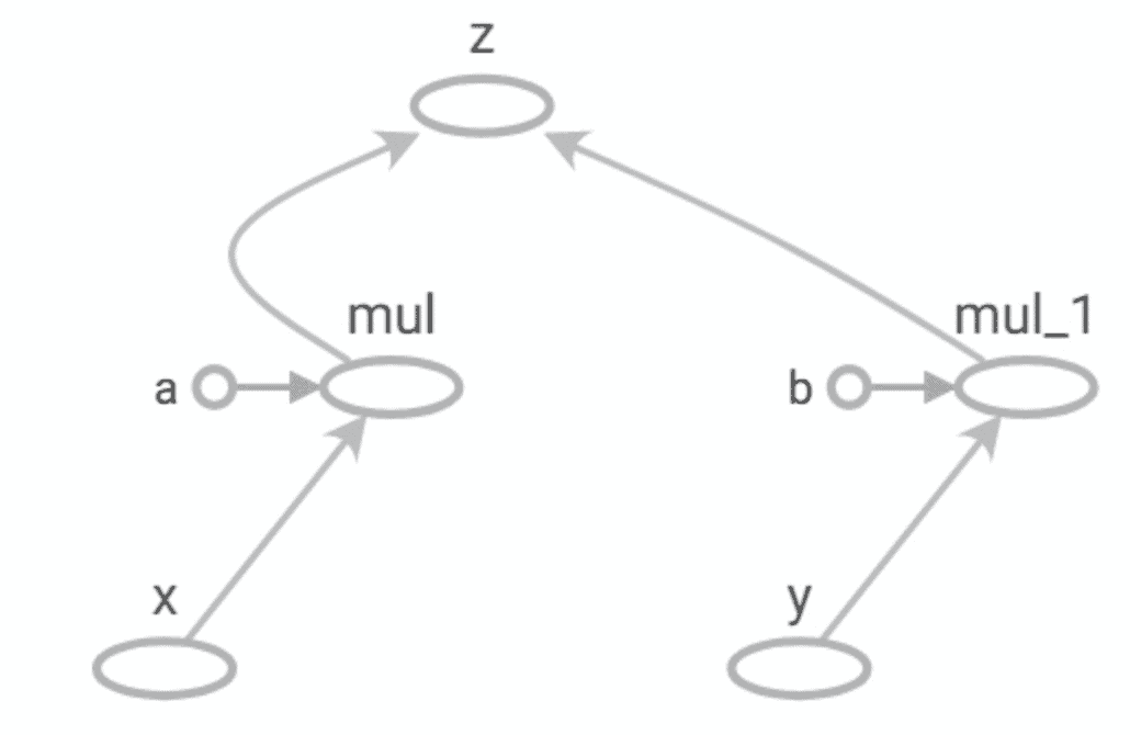
TensorBoard comes as part of TensorFlow installation.
Note the similarity between this and the manually drawn graph earlier!
6. Working with Session
We have now created a computational graph for our simple equation in TensorFlow Java API. But how do we run it? Before addressing that, let’s see what is the state of Graph we have just created at this point. If we try to print the output of our final Operation “z”:
System.out.println(z.output(0));This will result in something like:
<Add 'z:0' shape=<unknown> dtype=DOUBLE>This isn’t what we expected! But if we recall what we discussed earlier, this actually makes sense. The Graph we have just defined has not been run yet, so the tensors therein do not actually hold any actual value. The output above just says that this will be a Tensor of type Double.
Let’s now define a Session to run our Graph:
Session sess = new Session(graph)Finally, we are now ready to run our Graph and get the output we have been expecting:
Tensor<Double> tensor = sess.runner().fetch("z")
  .feed("x", Tensor.<Double>create(3.0, Double.class))
  .feed("y", Tensor.<Double>create(6.0, Double.class))
  .run().get(0).expect(Double.class);
System.out.println(tensor.doubleValue());
So what are we doing here? It should be fairly intuitive:
- Get a Runner from the Session
- Define the Operation to fetch by its name “z”
- Feed in tensors for our placeholders “x” and “y”
- Run the Graph in the Session
And now we see the scalar output:
21.0This is what we expected, isn’t it!
7. The Use Case for Java API
At this point, TensorFlow may sound like overkill for performing basic operations. But, of course, TensorFlow is meant to run graphs much much larger than this.
Additionally, the tensors it deals with in real-world models are much larger in size and rank. These are the actual machine learning models where TensorFlow finds its real use.
It’s not difficult to see that working with the core API in TensorFlow can become very cumbersome as the size of the graph increases. To this end, TensorFlow provides high-level APIs like Keras to work with complex models. Unfortunately, there is little to no official support for Keras on Java just yet.
However, we can use Python to define and train complex models either directly in TensorFlow or using high-level APIs like Keras. Subsequently, we can export a trained model and use that in Java using the TensorFlow Java API.
Now, why would we want to do something like that? This is particularly useful for situations where we want to use machine learning enabled features in existing clients running on Java. For instance, recommending caption for user images on an Android device. Nevertheless, there are several instances where we are interested in the output of a machine learning model but do not necessarily want to create and train that model in Java.
This is where TensorFlow Java API finds the bulk of its use. We’ll go through how this can be achieved in the next section.
8. Using Saved Models
We’ll now understand how we can save a model in TensorFlow to the file system and load that back possibly in a completely different language and platform. TensorFlow provides APIs to generate model files in a language and platform neutral structure called Protocol Buffer.
8.1. Saving Models to the File System
We’ll begin by defining the same graph we created earlier in Python and saving that to the file system.
Let’s see we can do this in Python:
import tensorflow as tf
graph = tf.Graph()
builder = tf.saved_model.builder.SavedModelBuilder('./model')
with graph.as_default():
  a = tf.constant(2, name='a')
  b = tf.constant(3, name='b')
  x = tf.placeholder(tf.int32, name='x')
  y = tf.placeholder(tf.int32, name='y')
  z = tf.math.add(a*x, b*y, name='z')
  sess = tf.Session()
  sess.run(z, feed_dict = {x: 2, y: 3})
  builder.add_meta_graph_and_variables(sess, [tf.saved_model.tag_constants.SERVING])
  builder.save()
As the focus of this tutorial in Java, let’s not pay much attention to the details of this code in Python, except for the fact that it generates a file called “saved_model.pb”. Do note in passing the brevity in defining a similar graph compared to Java!
8.2. Loading Models from the File System
We’ll now load “saved_model.pb” into Java. Java TensorFlow API has SavedModelBundle to work with saved models:
SavedModelBundle model = SavedModelBundle.load("./model", "serve");
Tensor<Integer> tensor = model.session().runner().fetch("z")
  .feed("x", Tensor.<Integer>create(3, Integer.class))
  .feed("y", Tensor.<Integer>create(3, Integer.class))
  .run().get(0).expect(Integer.class);
System.out.println(tensor.intValue());
It should by now be fairly intuitive to understand what the above code is doing. It simply loads the model graph from the protocol buffer and makes available the session therein. From there onward, we can pretty much do anything with this graph as we would have done for a locally-defined graph.
9. Conclusion
To sum up, in this tutorial we went through the basic concepts related to the TensorFlow computational graph. We saw how to use the TensorFlow Java API to create and run such a graph. Then, we talked about the use cases for the Java API with respect to TensorFlow.
In the process, we also understood how to visualize the graph using TensorBoard, and save and reload a model using Protocol Buffer.