

Mocking is an essential part of unit testing, and the Mockito library makes it easy to write clean and intuitive unit tests for your Java code.
Get started with mocking and improve your application tests using our Mockito guide:
Handling concurrency in an application can be a tricky process with many potential pitfalls. A solid grasp of the fundamentals will go a long way to help minimize these issues.
Get started with understanding multi-threaded applications with our Java Concurrency guide:
Spring 5 added support for reactive programming with the Spring WebFlux module, which has been improved upon ever since. Get started with the Reactor project basics and reactive programming in Spring Boot:
Since its introduction in Java 8, the Stream API has become a staple of Java development. The basic operations like iterating, filtering, mapping sequences of elements are deceptively simple to use.
But these can also be overused and fall into some common pitfalls.
To get a better understanding on how Streams work and how to combine them with other language features, check out our guide to Java Streams:
Explore Spring Boot 3 and Spring 6 in-depth through building a full REST API with the framework:
Yes, Spring Security can be complex, from the more advanced functionality within the Core to the deep OAuth support in the framework.
I built the security material as two full courses - Core and OAuth, to get practical with these more complex scenarios. We explore when and how to use each feature and code through it on the backing project.
You can explore the course here:
Spring Data JPA is a great way to handle the complexity of JPA with the powerful simplicity of Spring Boot.
Get started with Spring Data JPA through the guided reference course:
Refactor Java code safely — and automatically — with OpenRewrite.
Refactoring big codebases by hand is slow, risky, and easy to put off. That’s where OpenRewrite comes in. The open-source framework for large-scale, automated code transformations helps teams modernize safely and consistently.
Each month, the creators and maintainers of OpenRewrite at Moderne run live, hands-on training sessions — one for newcomers and one for experienced users. You’ll see how recipes work, how to apply them across projects, and how to modernize code with confidence.
Join the next session, bring your questions, and learn how to automate the kind of work that usually eats your sprint time.
Spring 5 added support for reactive programming with the Spring WebFlux module, which has been improved upon ever since. Get started with the Reactor project basics and reactive programming in Spring Boot:
1. Introduction
Project Reactor is a powerful library we can rely on when building fully non-blocking reactive applications in Java. Reactor introduces two composable reactive types: Flux and Mono.
With multi-core architectures being a commodity nowadays, being able to parallelize work easily is important. Regarding Flux, Project Reactor helps us do this by providing a special type, ParallelFlux, which exposes operators optimised for parallelised work.
In this tutorial, we’ll compare Flux and ParallelFlux, using a computationally intensive task to highlight their differences and the impact on performance in reactive applications.
2. Introduction to Flux
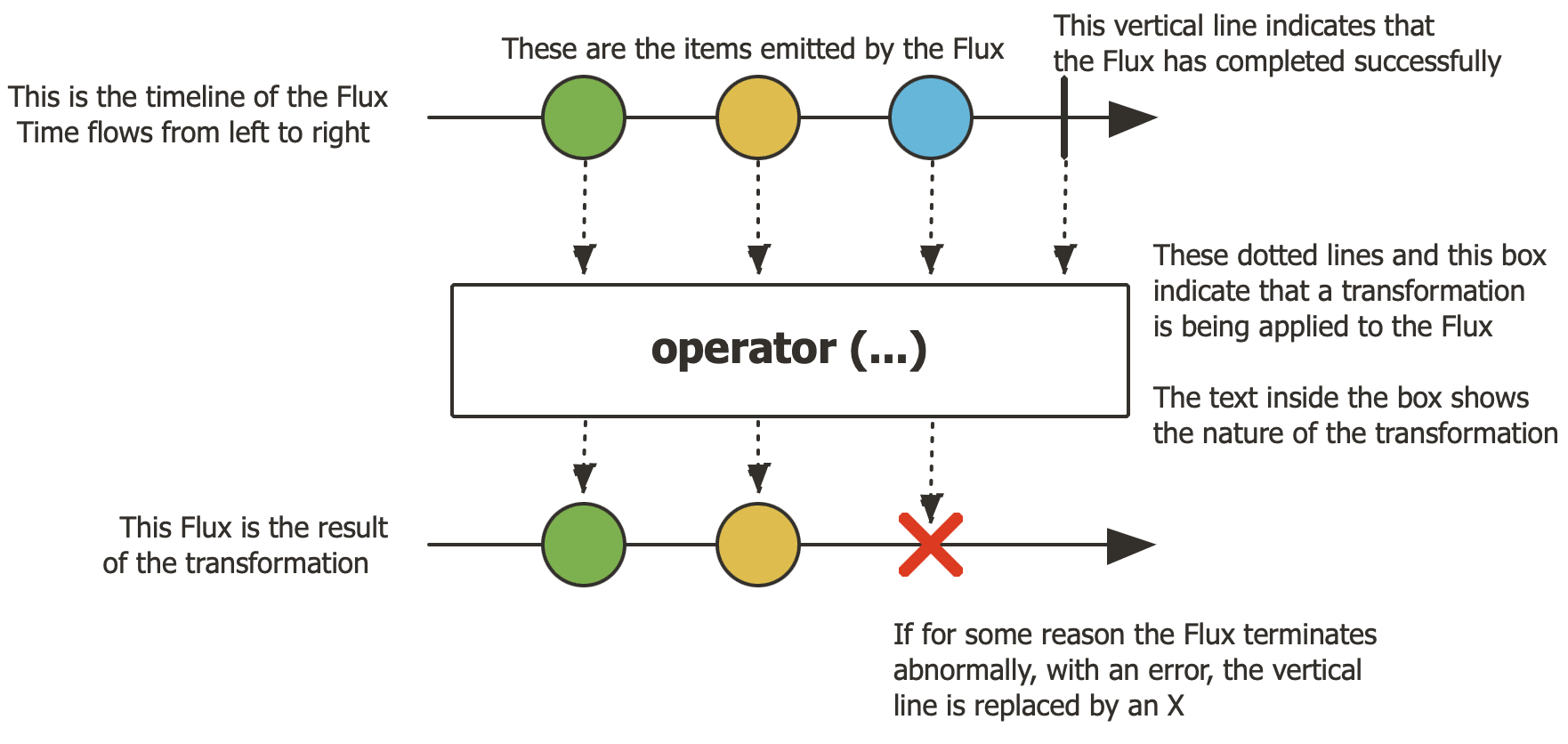
Flux is a fundamental type in Project Reactor, representing a reactive stream of 0 to N elements. Flux enables us to process data in an asynchronous and non-blocking manner, which is ideal for handling sequences such as database results or event streams, as illustrated in this diagram:
Here’s how to create a simple Flux:
Flux<Integer> flux = Flux.range(1, 10);By default, Flux operates sequentially on a single thread, but it can utilise schedulers for concurrency. Flux is straightforward and efficient for most reactive workflows, especially those involving I/O or small datasets.
3. Introduction to ParallelFlux
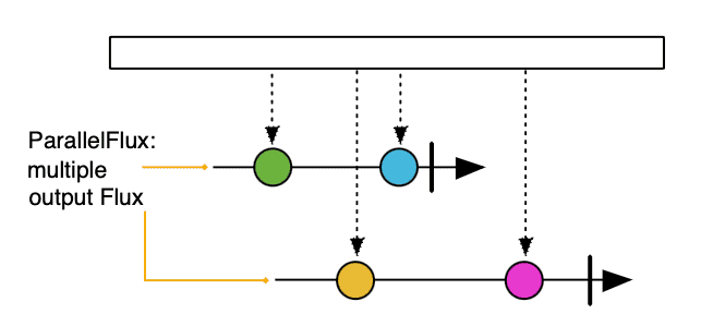
ParallelFlux extends Flux for parallel processing. ParallelFlux enables us to split a stream into multiple rails or sub-streams, each processed on a separate thread, making it suitable for CPU-intensive task, as illustrated in this diagram:
We can transform a Flux into a ParallelFlux using the parallel() operator along with runOn(Scheduler scheduler) by passing a Scheduler as a parameter:
Flux<Integer> flux = Flux.range(1, 10);
ParallelFlux<Integer> parallelFlux = flux.parallel(2).runOn(Schedulers.parallel());
ParallelFlux utilises multiple threads for faster computation, making it ideal for computationally intensive workloads.
4. Key Differences Between Flux and ParallelFlux
Let’s calculate Fibonacci numbers, a computationally intensive CPU-bound task, to showcase the performance differences between Flux and ParallelFlux, highlighting ParallelFlux’s strengths in parallel processing.
4.1. Fibonacci Calculation
We’ll process a list of integers, computing the Fibonacci number for each. The Fibonacci function is a recursive and computationally expensive function which simulates a real-world CPU-intensive task:
private long fibonacci(int n) {
    if (n <= 1) return n;
    return fibonacci(n - 1) + fibonacci(n - 2);
}
4.2. Flux Implementation for Fibonacci
Let’s implement the Flux version to process elements sequentially on a single thread:
Flux<Integer> flux = Flux.just(43, 44, 45, 47, 48)
  .map(n -> fibonacci(n));
This approach is simple but slower for CPU-bound workloads, as it processes each number one at a time.
4.3. ParallelFlux Implementation for Fibonacci
In the ParallelFlux version, we’ll split the stream into two rails, each running on a separate thread. By distributing the workload across two threads, ParallelFlux will reduce total execution time:
ParallelFlux<Integer> parallelFlux = Flux.just(43, 44, 45, 47, 48)
  .parallel(2)
  .runOn(Schedulers.parallel())
  .map(n -> fibonacci(n));
This demonstrates how ParallelFlux leverages multiple threads for faster computation.
4.4. Comparing Execution Time Between Flux and ParallelFlux
Here, to calculate the difference, we’ll measure the execution time for both Flux and ParallelFlux implementations when handling computationally expensive tasks using JMH.
Below is the test that performs the computation using Flux, which processes data sequentially:
@Test
public void givenFibonacciIndices_whenComputingWithFlux_thenCorrectResults() {
    Flux<Long> fluxFibonacci = Flux.just(43, 44, 45, 47, 48)
      .map(Fibonacci::fibonacci);

    StepVerifier.create(fluxFibonacci)
      .expectNext(433494437L, 701408733L, 1134903170L, 2971215073L, 4807526976L)
      .verifyComplete();
We measure the execution time for processing the Fibonacci sequence using Flux by running microbenchmarks with JMH, which provides reliable and repeatable performance measurements:
@Test
public void givenFibonacciIndices_whenComputingWithFlux_thenRunBenchMarks() throws IOException {
    Main.main(new String[] {
      "com.baeldung.reactor.flux.parallelflux.FibonacciFluxParallelFluxBenchmark.benchMarkFluxSequential",
         "-i", "3",
         "-wi", "2",
         "-f", "1"
    });
}
@Benchmark
public List<Long> benchMarkFluxSequential() {
Flux<Long> fluxFibonacci = Flux.just(43, 44, 45, 47, 48)
.map(Fibonacci::fibonacci);
return fluxFibonacci.collectList().block();
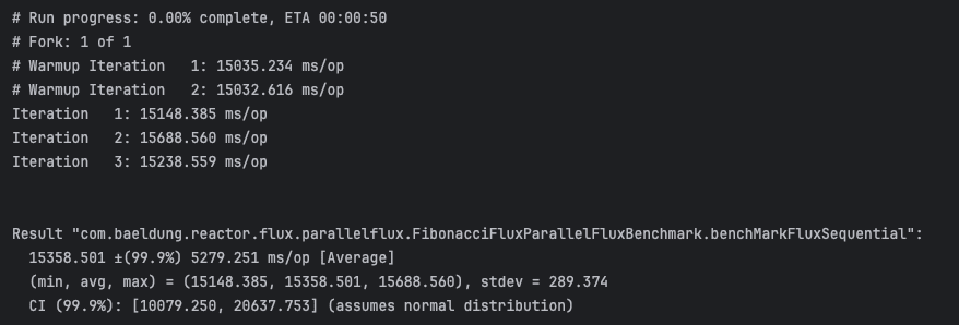
}The benchmark results shown below were collected on a multi-core machine and may vary slightly depending on system load and hardware configuration:

Next, we’ll compare this execution time against ParallelFlux implementation, where each computation is distributed across multiple threads, potentially speeding up total processing time depending on CPU availability and workload:
@Test
public void givenFibonacciIndices_whenComputingWithParallelFlux_thenCorrectResults() {
    ParallelFlux<Long> parallelFluxFibonacci = Flux.just(43, 44, 45, 47, 48)
      .parallel(3)
      .runOn(Schedulers.parallel())
      .map(Fibonacci::fibonacci);

    Flux<Long> sequencialParallelFlux = parallelFluxFibonacci.sequential();

    Set<Long> expectedSet = new HashSet<>(Set.of(433494437L, 701408733L, 1134903170L, 2971215073L, 4807526976L));

    StepVerifier.create(sequencialParallelFlux)
      .expectNextMatches(expectedSet::remove)
      .expectNextMatches(expectedSet::remove)
      .expectNextMatches(expectedSet::remove)
      .expectNextMatches(expectedSet::remove)
      .expectNextMatches(expectedSet::remove)
      .verifyComplete();
Similar to what we did for Flux, we measure the time it takes to process the Fibonacci sequence using ParallelFlux with JMH for comparison with the sequential Flux version:
@Benchmark
public List<Long> benchMarkParallelFluxSequential() {
    ParallelFlux<Long> parallelFluxFibonacci = Flux.just(43, 44, 45, 47, 48)
      .parallel(3)
      .runOn(Schedulers.parallel())
      .map(Fibonacci::fibonacci);

    return parallelFluxFibonacci.sequential().collectList().block();
}
@Test
public void givenFibonacciIndices_whenComputingWithParallelFlux_thenRunBenchMarks() throws IOException {
Main.main(new String[] {
"com.baeldung.reactor.flux.parallelflux.FibonacciFluxParallelFluxBenchmark.benchMarkParallelFluxSequential",
"-i", "3",
"-wi", "2",
"-f", "1"
});
}The JMH benchmark result below captures the total execution time in milliseconds, showcasing the benefit of parallel execution. Despite concurrent processing, each Fibonacci index is computed exactly once and emitted once:
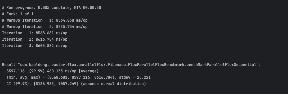

Our tests show that, on a typical multi-core CPU, ParallelFlux is significantly faster than Flux for CPU-bound tasks.
5. Schedulers in Project Reactor
We rely on schedulers to control which threads handle our reactive streams. Schedulers are essential for controlling concurrency in both Flux and ParallelFlux.
Schedulers.parallel() is optimized for CPU-bound tasks, utilising a fixed thread pool size equal to the number of available CPU cores. Schedulers.boundedElastic() is optimized for I/O-bound tasks which can dynamically grow the thread pool as needed.
ParallelFlux always requires a scheduler to define where each rail should run, typically using Schedulers.parallel() for compute-heavy workloads. Flux can also use schedulers such as publishOn(Schedulers.boundedElastic()) to introduce concurrency and enhance responsiveness for I/O operations, even without parallel processing.
Always make sure to choose the scheduler that matches your workload: Schedulers.parallel() for CPU-bound, Schedulers.boundedElastic() for I/O-bound. This ensures efficient and responsive execution, whether using Flux or ParallelFlux.
6. Choosing Between Flux and ParallelFlux
We choose between Flux and ParallelFlux based on the type of workload in our reactive pipeline.
Flux should be used for I/O-bound tasks like REST calls or database access, where parallelism adds little benefit. It’s also ideal for small datasets or lightweight operations where sequential processing is fast enough.
ParallelFlux should be used for CPU-intensive tasks, where parallelism reduces execution time. It’s also ideal for large datasets where distributing work across cores enhances performance.
Our test highlights how ParallelFlux improves performance for compute-heavy tasks while Flux remains simpler and more efficient for lightweight or I/O-driven workflows.
7. Practical Pitfalls and Best Practices
In this section, we’ll address common pitfalls and best practices when using ParallelFlux, using simple code examples and tests to validate these claims.
7.1. Pitfalls With ParallelFlux
When we use ParallelFlux, we introduce thread management overhead. For small or lightweight tasks, this overhead can actually slow us down compared to using Flux.
Using more rails than available CPU cores, can cause thread contention, such as using eight rails on a 4-core machine, resulting in degraded performance rather than improvements.
By default, ParallelFlux doesn’t preserve order, which can be problematic in order-sensitive workflows unless ordered() or post-processing is applied.
Let’s create a simple function to convert a small list of string IDs to uppercase using ParallelFlux. This illustrates how ParallelFlux processes elements in parallel without guaranteeing output order.
To better observe this behaviour, we run the same test repeatedly 5 times using JUnit’s RepeatedTest annotation:
@RepeatedTest(5)
public void givenListOfIds_whenComputingWithParallelFlux_OrderChanges() {
    ParallelFlux<String> parallelFlux = Flux.just("id1", "id2", "id3")
      .parallel(2)
      .runOn(Schedulers.parallel())
      .map(String::toUpperCase);

    List<String> emitted = new CopyOnWriteArrayList<>();

    StepVerifier.create(parallelFlux.sequential().doOnNext(emitted::add))
      .expectNextCount(3)
      .verifyComplete();

    log.info("ParallelFlux emitted order: {}", emitted);
}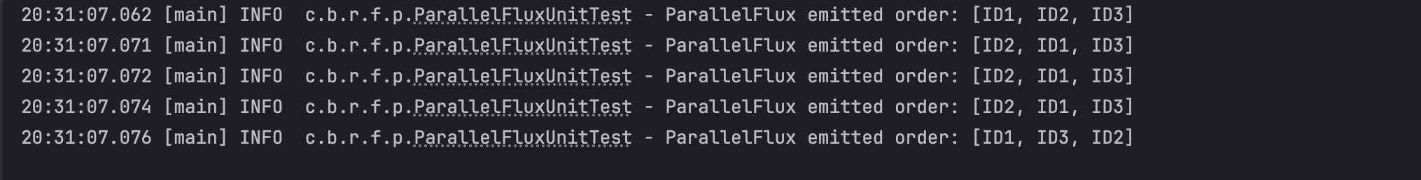
Although each run processes the same input, the log output from all 5 runs shows that the order of emitted elements may vary between executions. This is because ParallelFlux executes work concurrently across threads, and without any ordering constraints, the final sequence is not deterministic.
7.2. Best Practices With ParallelFlux
For CPU-bound tasks, we recommend to use Schedulers.parallel(), which is backed by a fixed-size thread pool equal to the number of available CPU cores.
This ensures efficient parallel execution without overwhelming the system.
To fully leverage available processing power, set the number of rails to match the number of CPU cores. You can retrieve this information using Runtime.getRuntime().availableProcessors() to adapt to the machine’s capacity dynamically.
The following example shows setting the number of rails to match CPU cores and using Schedulers.parallel() for efficient parallel execution of Fibonacci calculations with ParallelFlux:
ParallelFlux<Long> parallelFlux = Flux.just(40, 41, 42, 43, 44, 45, 46, 47, 48, 49)
    .parallel(Runtime.getRuntime().availableProcessors())
    .runOn(Schedulers.parallel())
    .map(n -> fibonacci(n));
8. Conclusion
In this article, we compared Flux and ParallelFlux using the Fibonacci algorithm, which is a computationally intensive task. We also explored when to use Flux versus ParallelFlux, highlighting their differences and discussing best practices and pitfalls regarding ParallelFlux.


