

Learn through the super-clean Baeldung Pro experience:
>> Membership and Baeldung Pro.
No ads, dark-mode and 6 months free of IntelliJ Idea Ultimate to start with.
Learn through the super-clean Baeldung Pro experience:
>> Membership and Baeldung Pro.
No ads, dark-mode and 6 months free of IntelliJ Idea Ultimate to start with.
In this tutorial, we’ll look at dedicated Linux benchmarking tools for both graphical and command-line environments.
Further, we’ll see examples that don’t refer to any particular Linux distribution. Because of this, we won’t cover how to install the various tools, as the installation procedures are often distribution-dependent.
Benchmarks can help evaluate our machine’s performance during specific tasks. We can also use benchmarks to compare two machines or compare our computer with a scores database.
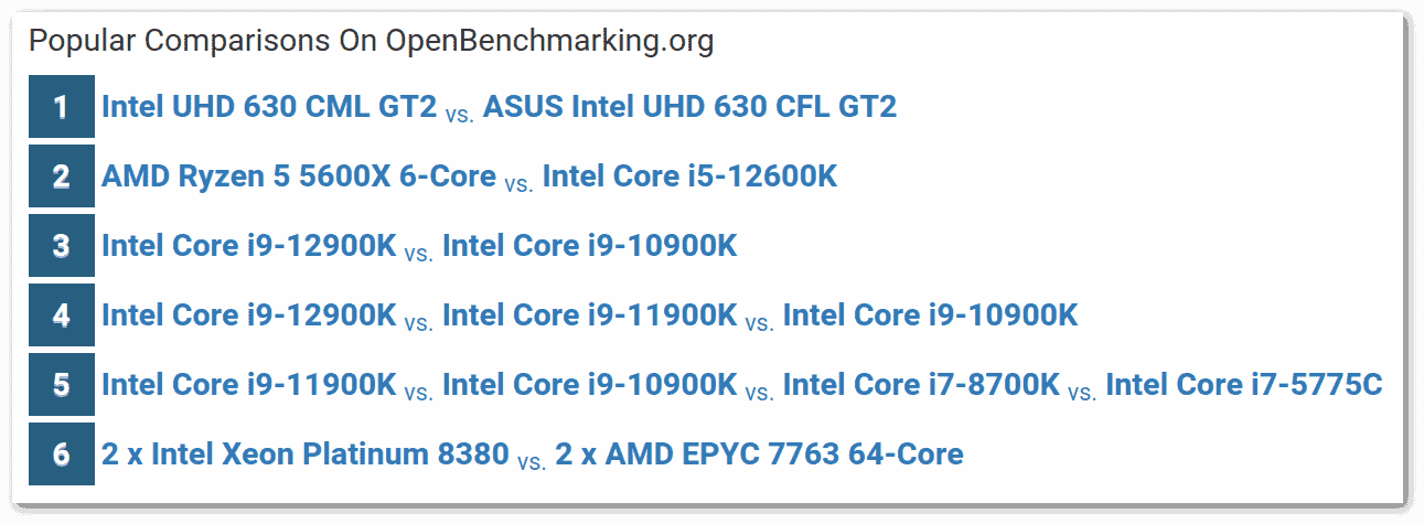
We can use the rankings already published on the web to choose which hardware to buy, as in this example provided by openbenchmarking.org:
 Sometimes we need benchmarking to optimize system performance and remove bottlenecks caused by hardware or software, such as problematic updates, regressions, and buggy drivers. Benchmarking also comes in handy to evaluate the characteristics of a virtual private server (VPS).
Stressing is similar but not equivalent to benchmarking in that we don’t need it to evaluate performance. Instead, it helps us uncover bugs under heavy load and assess how well our systems scale. In general, we can turn any benchmark into a stressing tool simply by increasing its execution time significantly.
First, let’s avoid using dd to test the speed of writing zeros or random data. dd is popular because it comes preinstalled on almost all Linux distributions, but it can give us unrealistic results. In fact, some filesystems and disks handle writing zeros and other compressible data in a particular way, which will cause benchmark results to be too high. On the other hand, if we use a random generator, we will measure that one and not the disk.
Let’s also keep in mind that benchmark results can be affected by:
An additional problem is figuring out what we want to measure. We can push our disks to unrealistic edge cases that will never occur in our workstation or server. Still, unlikely cases rarely provide useful performance data. The best benchmark criterion is our actual workload.
We should also be careful not to subject our disks to overly stressful benchmarks. All disks have some wear with writing, so running tests that repeat writing in the same locations thousands of times can shorten their lives.
Furthermore, some devices may have intelligent wear-leveling algorithms that use the internal cache to replace quickly rewritten data without touching the disk. Of course, this internal caching will cause us to see more optimistic results than the real ones.
Beyond the tool used, the measures of interest for disk benchmarking are:
Let’s try some tools after premising the possible troubles.
We have already discussed hdparm to distinguish between SSD and HDD. hdparm is a tool for collecting and manipulating the low-level parameters of SATA/PATA/SAS and older IDE storage devices. It also contains a benchmark mode we can invoke with the -t flag, even on a disk with mounted partitions:
# hdparm -t /dev/sda
/dev/sda:
 Timing buffered disk reads: 1512 MB in  3.00 seconds = 503.87 MB/sec
This test indicates how fast the disk can sustain sequential data reads without any filesystem overhead and without prior caching since hdparm automatically flushes it.
According to the manual page, we’d best repeat this benchmark two or three times on a system with no other active processes and at least a couple of megabytes of free memory.
Let’s try to compare two disks by repeating the measurements three times. In this example, sda is an SSD, and sdb is an HDD:
# for i in {1..3}; do hdparm -t /dev/sda; hdparm -t /dev/sdb; doneSo we see that sda is 3.6 times faster than sdb in reading:
/dev/sda:
 Timing buffered disk reads: 1508 MB in  3.00 seconds = 502.18 MB/sec

/dev/sdb:
 Timing buffered disk reads: 420 MB in  3.00 seconds = 140.00 MB/sec

/dev/sda:
 Timing buffered disk reads: 1510 MB in  3.00 seconds = 502.52 MB/sec

/dev/sdb:
 Timing buffered disk reads: 426 MB in  3.01 seconds = 141.39 MB/sec

/dev/sda:
 Timing buffered disk reads: 1512 MB in  3.00 seconds = 503.66 MB/sec

/dev/sdb:
 Timing buffered disk reads: 424 MB in  3.01 seconds = 140.85 MB/sec
Comparing the value of sda (502MB/s) with the performance metrics of openbenchmarking.org, we notice that the performance is excellent, among the highest values.
fio stands for Flexible I/O Tester and refers to a tool for measuring I/O performance. With fio, we can set our workload to get the type of measurement we want.
The –filename flag allows us to test a block device, such as /dev/sda, or just a file. However, writing to a block device will overwrite it, making the data it contains unusable. On the other hand, we can safely use a device name along with the –readonly option.
Let’s start with a simple example, similar to the one with hdparm: measuring the sequential read speed of /dev/sda and /dev/sdb for three seconds (–runtime=3). We name the test with –name, and –rw decides between sequential (–rw=read) or random I/O access:
# fio --filename=/dev/sda --readonly --rw=read --name=TEST --runtime=3The output is very verbose, but we’re interested in this line:
read: IOPS=128k, BW=498MiB/s (523MB/s)(1496MiB/3001msec)The bandwidth (523MB/s) is very similar to the one from hdparm (502MB/s). We notice the same with /dev/sdb and its bandwidth of 147MB/s, compared to hdparm’s 141MB/s.
Let’s see all the options for –rw:
The options to fio and their possible combinations are many and possibly confusing, as shown on the man page. That’s why Oracle published sample FIO commands for block volume performance tests, covering the most common scenarios.
Once we find the workload we are interested in, we can test with a job file without the need for command-line options. So, we can save the previous example in test.fio:
[global]
runtime=3
name=TEST
rw=read

[job1]
filename=/dev/sda
We can execute the test again, optionally adding –readonly for extra safety:
# fio --readonly test.fioLet’s check the actual results in a more user-friendly environment.
gfio is a GTK+ based GUI frontend for fio. In some cases, such as accessing /dev/sda, it may require root permissions to work correctly, same as fio. It provides us with detailed reports and charts, plus an editor to automatically generate or modify job files.
The following screenshots are with test.fio above, but from a virtual machine:
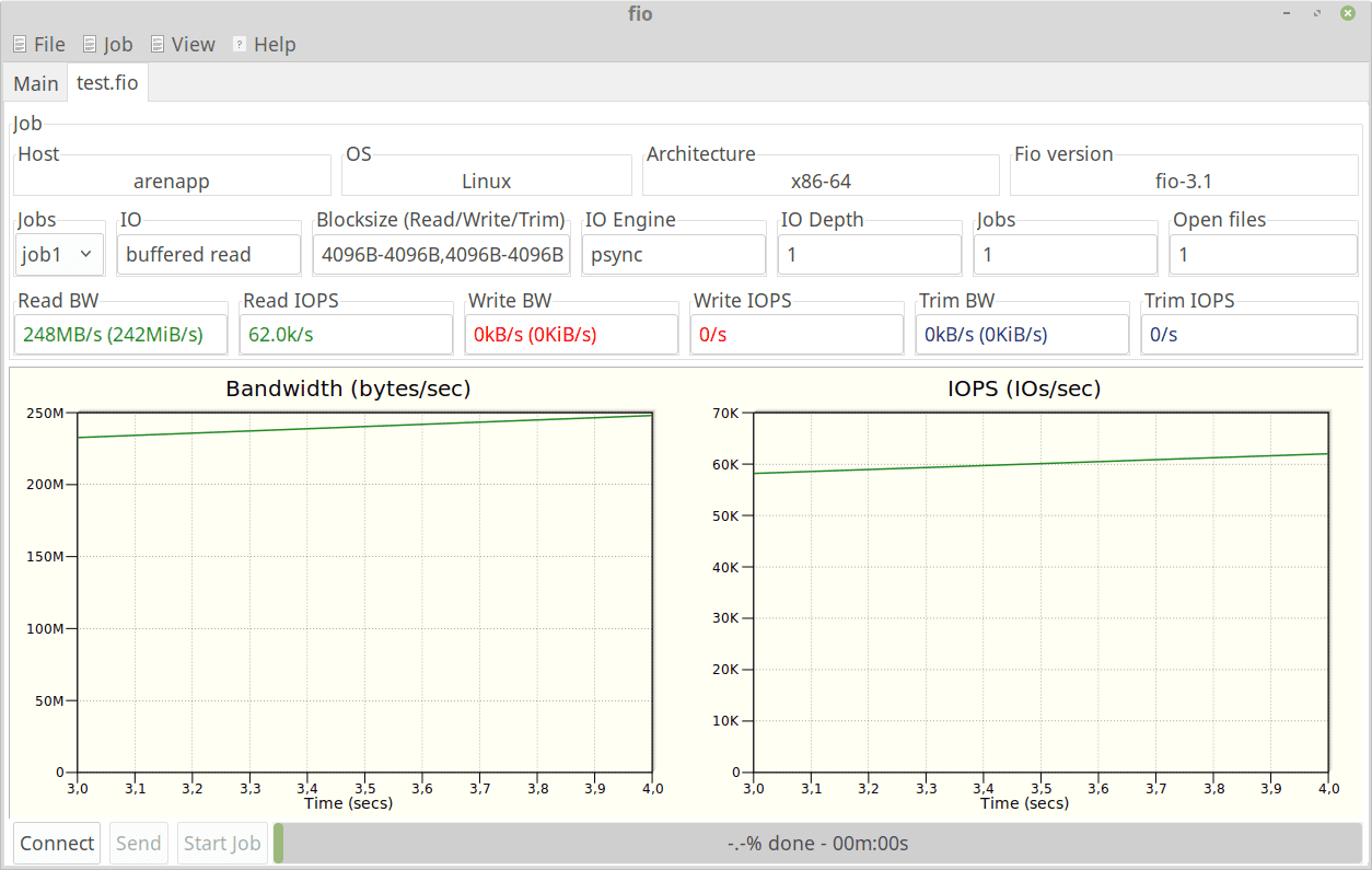
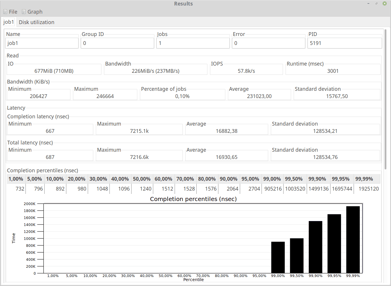
There’s a 55% degradation in performance within this virtual machine installed on /dev/sda compared to the host. For instance, bandwidth dropped from 523MB/s to 237MB/s, total read IO operations dropped from 1496MiB/3001msec to 677MiB/3001msec, IOPS dropped from 128k/s to 57.8k/s.
We can refer to this comprehensive documentation for all other information provided by both fio and gfio.
sysbench is a modular, cross-platform, and multi-threaded benchmark tool for evaluating parameters, important for running a database under intensive load. Luckily, sysbench interacts directly with the operating system, so it’s independent of any particular database.
First, we have to create a set of test files as I/O targets. For this purpose, we use the fileio parameter of sysbench to perform I/O testing. The –file-total-size flag indicates the total size of test files to be created locally. We execute prepare before the actual run:
$ mkdir tempBenchmarkFiles
$ cd tempBenchmarkFiles
$ sysbench fileio --file-total-size=50G prepare
In this example, the tool will create 128 files of about 400MB each, filled with zeroes. Then, we can actually run the disk benchmark.
For instance, let’s execute a random read/write workload:
$ sysbench --file-total-size=50G --file-test-mode=rndrw --file-extra-flags=direct fileio runsysbench 1.0.18 (using system LuaJIT 2.1.0-beta3) Running the test with following options: Number of threads: 1 Initializing random number generator from current time Extra file open flags: directio 128 files, 400MiB each 50GiB total file size Block size 16KiB Number of IO requests: 0 Read/Write ratio for combined random IO test: 1.50 Periodic FSYNC enabled, calling fsync() each 100 requests. Calling fsync() at the end of test, Enabled. Using synchronous I/O mode Doing random r/w test Initializing worker threads... Threads started! File operations: reads/s: 1310.23 writes/s: 873.52 fsyncs/s: 2796.86 Throughput: read, MiB/s: 20.47 written, MiB/s: 13.65 General statistics: total time: 10.0194s total number of events: 49791 Latency (ms): min: 0.06 avg: 0.20 max: 22.64 95th percentile: 0.45 sum: 9960.44 Threads fairness: events (avg/stddev): 49791.0000/0.00 execution time (avg/stddev): 9.9604/0.00
The –file-extra-flags=direct option tells sysbench to use direct I/O, which will bypass the page cache. This choice ensures that the test interacts with the disk and not with the main memory. We can also set a duration in seconds with the –time flag.
–file-test-mode accepts the following workloads:
Finally, let’s remove the temporary files:
$ sysbench fileio cleanupThe man page is a bit concise. We can also delve into sysbench-manual.pdf, a comprehensive manual.
The central aspect of CPU benchmarking is choosing which computations to measure the execution time of. In theory, we wouldn’t need any particular software.
For instance, we could decide to compile the same software on different machines, or hash hundreds of heavy files, and compare the times. Of course, the boundary conditions must be the same: operating system, files, options used to compile or hash, and so on. Furthermore, we could create a small Bash script that repeats some calculations a million times. However, this approach can be good only if we are interested in a specific task.
For more general CPU testing, Geekbench seems quite complete. It’s a command-line tool that tests the CPU against the following single-core and multi-core tests:
It’s proprietary software with a free version. At the end of the benchmark, Geekbench uploads the results online and gives us a link like this one to view them.
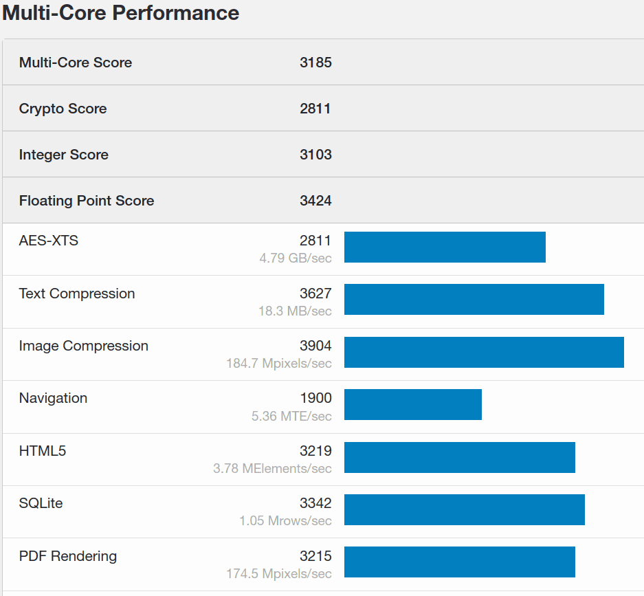
We can then compare our CPUs with the Geekbench benchmarks database. Again, we can also make a comparison with the performance metrics from openbenchmarking.org, noting that the result shown in the screenshot is very low.
One might think that evaluating video card performance serves almost exclusively for gaming. It doesn’t.
For example, let’s think about Augmented Reality (AR) or immersion in Virtual Reality (VR). There’s more to building the perfect VR experience than choosing the right VR headset or the most effective AR software. One of the essential tools in ensuring we get a genuinely realistic VR experience is our GPU.
We can also think about Machine Learning (ML), a subset of Artificial Intelligence (AI). ML is the ability of computer systems to learn to make decisions and predictions from observations and data. A GPU is a specialized processing unit with enhanced mathematical computation capability, making it ideal for ML.
Another interesting example is the mining of cryptocurrencies, like Bitcoin or Ethereum. Mining is the process of creating a block of transactions and adding it to the blockchain. We need dedicated hardware to solve complex mathematical puzzles to mine, such as an excellent graphics card. For instance, the VRAM (Video RAM) requirement to mine Ethereum coins is more than 4GB. But this is only a minimum requirement.
From these observations, it is clear that GPU benchmarking isn’t enough if we plan to run specific tasks. In the examples suggested here, we must thoroughly investigate the needed hardware.
Usually, GPU benchmarking involves the on-the-fly creation of more or less complex moving images and the measurement of frames per second (fps).
Generally, the higher the fps value, the better. High values mean that the video card can render the 3D scene without particular difficulties. Low values mean that the complexity of the graphic work is too much for the video card. For the human eye, a movie at 60fps is desirable.
Let’s remember that low benchmark scores don’t necessarily indicate a faulty GPU. Old drivers, open-source drivers instead of proprietary drivers (or vice versa), overheating, or power issues can cause low scoring.
glmark2 has a suite of scenes to measure many aspects of OpenGL (ES) 2.0 performance. We can configure how each scene is rendered through a set of options. It takes a few minutes to complete the test and provide a score. Here is one of the scenes:
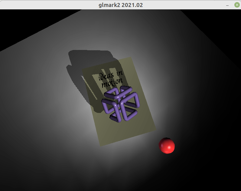
In one of our virtual machines, this comprehensive test provided the following logging and final score:
$ glmark2
=======================================================
    glmark2 2014.03+git20150611.fa71af2d
=======================================================
    OpenGL Information
    GL_VENDOR:     VMware, Inc.
    GL_RENDERER:   SVGA3D; build: RELEASE;  LLVM;
    GL_VERSION:    2.1 Mesa 20.0.8
=======================================================
[build] use-vbo=false: FPS: 615 FrameTime: 1.626 ms
[build] use-vbo=true: FPS: 2364 FrameTime: 0.423 ms
[texture] texture-filter=nearest: FPS: 1567 FrameTime: 0.638 ms
[texture] texture-filter=linear: FPS: 1546 FrameTime: 0.647 ms
[texture] texture-filter=mipmap: FPS: 1525 FrameTime: 0.656 ms
[shading] shading=gouraud: FPS: 1563 FrameTime: 0.640 ms
[shading] shading=blinn-phong-inf: FPS: 1491 FrameTime: 0.671 ms
[shading] shading=phong: FPS: 1338 FrameTime: 0.747 ms
[shading] shading=cel: FPS: 1334 FrameTime: 0.750 ms
[bump] bump-render=high-poly: FPS: 1443 FrameTime: 0.693 ms
[bump] bump-render=normals: FPS: 1395 FrameTime: 0.717 ms
[bump] bump-render=height: FPS: 1279 FrameTime: 0.782 ms
[effect2d] kernel=0,1,0;1,-4,1;0,1,0;: FPS: 1420 FrameTime: 0.704 ms
[effect2d] kernel=1,1,1,1,1;1,1,1,1,1;1,1,1,1,1;: FPS: 1427 FrameTime: 0.701 ms
[pulsar] light=false:quads=5:texture=false: FPS: 610 FrameTime: 1.639 ms
[desktop] blur-radius=5:effect=blur:passes=1:separable=true:windows=4: FPS: 247 FrameTime: 4.049 ms
[desktop] effect=shadow:windows=4: FPS: 220 FrameTime: 4.545 ms
[buffer] columns=200:interleave=false:update-dispersion=0.9:update-fraction=0.5:update-method=map: FPS: 184 FrameTime: 5.435 ms
[buffer] columns=200:interleave=false:update-dispersion=0.9:update-fraction=0.5:update-method=subdata: FPS: 233 FrameTime: 4.292 ms
[buffer] columns=200:interleave=true:update-dispersion=0.9:update-fraction=0.5:update-method=map: FPS: 235 FrameTime: 4.255 ms
[ideas] speed=duration: FPS: 668 FrameTime: 1.497 ms
[jellyfish] <default>: FPS: 1734 FrameTime: 0.577 ms
Error: SceneTerrain requires Vertex Texture Fetch support, but GL_MAX_VERTEX_TEXTURE_IMAGE_UNITS is 0
[terrain] <default>: Unsupported
[shadow] <default>: FPS: 1023 FrameTime: 0.978 ms
[refract] <default>: FPS: 868 FrameTime: 1.152 ms
[conditionals] fragment-steps=0:vertex-steps=0: FPS: 1715 FrameTime: 0.583 ms
[conditionals] fragment-steps=5:vertex-steps=0: FPS: 1463 FrameTime: 0.684 ms
[conditionals] fragment-steps=0:vertex-steps=5: FPS: 1425 FrameTime: 0.702 ms
[function] fragment-complexity=low:fragment-steps=5: FPS: 1432 FrameTime: 0.698 ms
[function] fragment-complexity=medium:fragment-steps=5: FPS: 1405 FrameTime: 0.712 ms
[loop] fragment-loop=false:fragment-steps=5:vertex-steps=5: FPS: 1357 FrameTime: 0.737 ms
[loop] fragment-steps=5:fragment-uniform=false:vertex-steps=5: FPS: 1269 FrameTime: 0.788 ms
[loop] fragment-steps=5:fragment-uniform=true:vertex-steps=5: FPS: 1311 FrameTime: 0.763 ms
=======================================================
                                  glmark2 Score: 1178
=======================================================
Based on performance metrics for 800×600 pixels, reported on openbenchmarking.org, this score is too low for a decent performance. In comparison, the median score is 3172, and the mid-tier score is 7765.
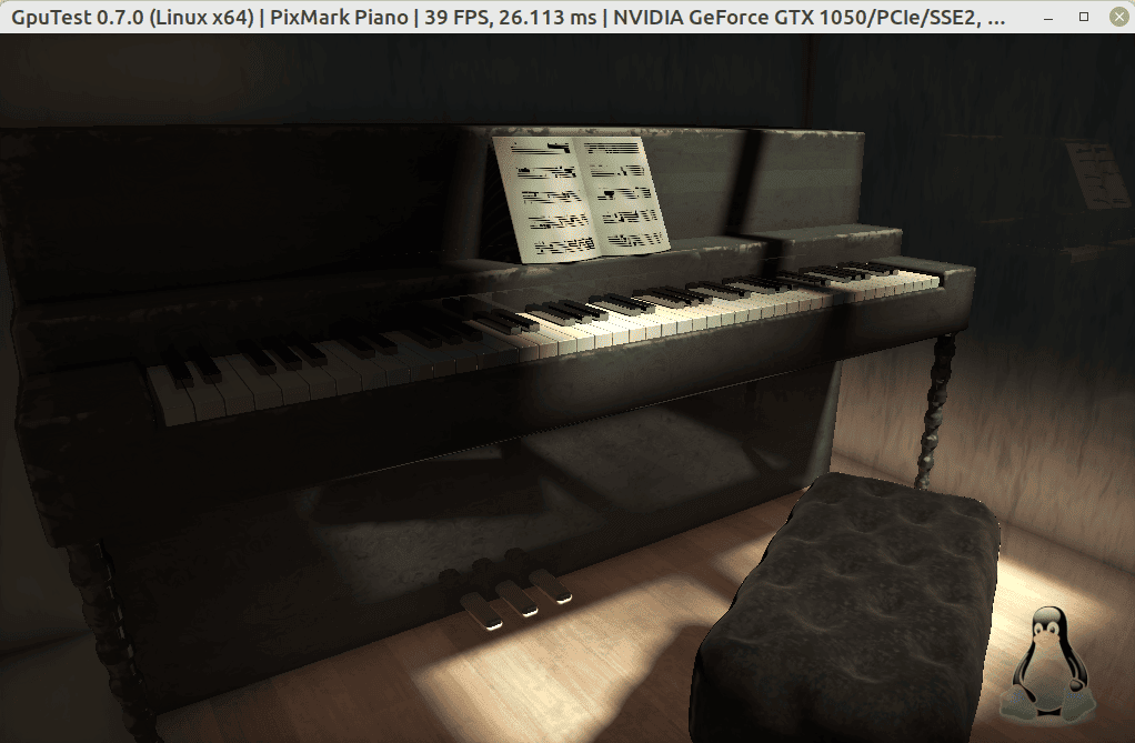
geeks3d’s GpuTest is a cross-platform freeware OpenGL benchmark. It contains several GPU benchmarks (furmark, gimark, pixmark, and others) and an exhaustive README.txt.
The following screenshot is an example of the pixmark benchmark. Note, that the title bar shows the fps in real-time. When the test finishes, it also gives us a score, which we can compare with this updated score database.
In our case, the furmark score is 2833:
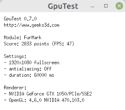
Comparing our result with the top-20 scores, which are between 85324 and 180278, we understand that our GPU has severe limitations.
We could think that the same type of memory sticks would perform similarly on two different machines, but that is rarely the case. RAM performance depends more on the CPU and motherboard than the memory type and speed. On the other hand, the amount of RAM is a deciding factor in general system performance.
With that in mind, let’s benchmark the RAM with sysbench.
By default, the tool performs a writing test unless we use –memory-oper=read:
$ sysbench memory --memory-access-mode=rnd run
sysbench 1.0.18 (using system LuaJIT 2.1.0-beta3)

Running the test with following options:
Number of threads: 1
Initializing random number generator from current time


Running memory speed test with the following options:
  block size: 1KiB
  total size: 102400MiB
  operation: write
  scope: global

Initializing worker threads...

Threads started!

Total operations: 20126299 (2012308.75 per second)

19654.59 MiB transferred (1965.15 MiB/sec)


General statistics:
    total time:                          10.0001s
    total number of events:              20126299

Latency (ms):
         min:                                    0.00
         avg:                                    0.00
         max:                                    0.04
         95th percentile:                        0.00
         sum:                                 8260.00

Threads fairness:
    events (avg/stddev):           20126299.0000/0.00
    execution time (avg/stddev):   8.2600/0.00
The possible values for –memory-access-mode are seq (sequential access, by default) and rnd (random access). To see all the options, we can use sysbench memory help.
Comparing the previously obtained value (1965.15 MiB/sec) with the performance metrics of openbenchmarking.org, the result seems below the minimum value. However, the values from openbenchmarking.org likely refer to a sequential write-only test, which we can run with sysbench memory run. In that case, we get 5847.83 MiB/sec, which is very close to the median value.
Moreover, we can assess whether the RAM performance in the virtual machine is lower than that of its host:
$ sysbench memory --memory-access-mode=rnd run
sysbench 1.0.11 (using system LuaJIT 2.1.0-beta3)

Running the test with following options:
Number of threads: 1
Initializing random number generator from current time


Running memory speed test with the following options:
  block size: 1KiB
  total size: 102400MiB
  operation: write
  scope: global

Initializing worker threads...

Threads started!

Total operations: 17710992 (1770824.00 per second)

17295.89 MiB transferred (1729.32 MiB/sec)


General statistics:
    total time:                          10.0001s
    total number of events:              17710992

Latency (ms):
         min:                                  0.00
         avg:                                  0.00
         max:                                  1.02
         95th percentile:                      0.00
         sum:                               7772.77

Threads fairness:
    events (avg/stddev):           17710992.0000/0.00
    execution time (avg/stddev):   7.7728/0.00
In this case, we can see a pretty insignificant (10%) degradation.
In this tutorial, we explored some tools to measure the performance of the hard disk, CPU, GPU, and RAM. Before running any tests, we should imagine our actual workload and what we want to measure.
This way, we can discover any weaknesses or misconfigurations of our computer. We can also make comparisons and estimate the actual performance of rented machines, such as VPSes.