The Wavelet Transform | Baeldung on Computer Science

1. Introduction

Signals appear across various domains, from audio recordings and heartbeats to seismic waves and financial trends. Understanding what’s happening in these signals, and when, is critical in many fields.

In this tutorial, we’ll explore the wavelet transform, a mathematical technique for analyzing signals at different scales. We’ll also understand the intuition behind wavelets, look into the types of transforms, and walk through an example using PyWavelets.

2. Signal Decomposition

The wavelet transform allows us to study a signal at multiple levels of detail. It does this by breaking the signal into smaller components using short-lived oscillating functions called wavelets. These wavelets are designed to capture both rapid changes and slower trends within a signal. Unlike the Fourier transform, which only provides frequency information, the wavelet transform gives both time and frequency insights:

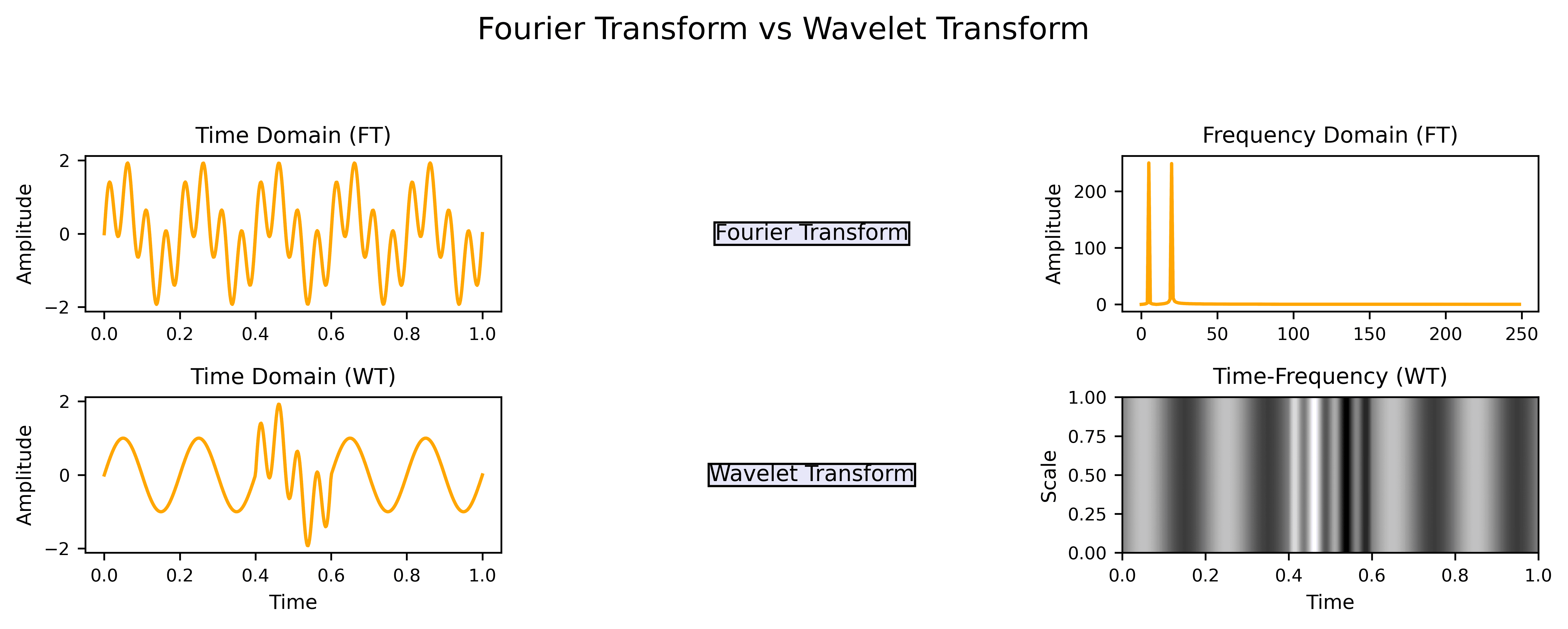
The Fourier transform is great for signals whose frequency content doesn’t change over time. However, wavelets are especially useful when working with real-world signals that aren’t uniform over time. Whether we’re analyzing a sudden voltage drop in an ECG or a brief sound in an audio file, we need tools to focus on specific signal moments.

3. Types of Wavelet Transform

There are two main types of wavelet transforms: continuous and discrete.

3.1. Continuous Wavelet Transform (CWT)

The CWT slides a scaled version of a mother wavelet across the signal, a small, oscillating function that serves as the basic shape for analysis. At each step, we compute how closely the wavelet matches the signal:

$W(a, b) = \int_{-\infty}^{+\infty} x(t)\, \psi^* \left( \frac{t - b}{a} \right) dt$

In this equation, $W(a, b)$ gives us the wavelet coefficient at scale $a$ and time shift $b$ . The function $x(t)$ is the original signal, and $\psi^*$ is the complex conjugate of the mother wavelet $\psi$ .

The complex conjugate ensures that the inner product captures both the amplitude and phase alignment between the wavelet and the signal. For real-valued wavelets, $\psi^* = \psi$ , so the expression simplifies accordingly.

The variable $a$ controls the scale:

Small values reveal high-frequency details, while large ones capture low-frequency trends. The shift $b$ slides the wavelet across the signal. So, the integral $W(a, b)$ tells us how well the scaled and shifted wavelet $\psi \left( \frac{t - b}{a} \right)$ matches the signal $x(t)$ .

The wavelet captures fine, high-frequency details when $a$ is small. When $a$ is large, it captures slower, broader features. The result is a time-frequency map that shows where different patterns occur.

Since the CWT computes coefficients at every possible scale and time shift, it produces many closely related or redundant values. This fine-grained analysis is robust but requires more memory and computation.

3.2. Discrete Wavelet Transform (DWT)

The discrete wavelet transform (DWT) produces a more compact and efficient signal representation. The process involves working with selected scales and positions, usually powers of two.

Here, we split the signal at each level into approximation coefficients that capture low-frequency content and detail coefficients that retain high-frequency components.

Mathematically, we express the DWT as:

$W_{j, k} = \sum_{n} x[n] \cdot \psi_{j, k}[n]$

Here, $x[n]$ is the input signal, and $\psi_{j, k}[n]$ is the discrete wavelet function at scale $j$ and position $k$ . The result $W_{j, k}$ gives us the wavelet coefficient at that scale and location.

We repeat this process on the approximation part, creating a multi-level decomposition:

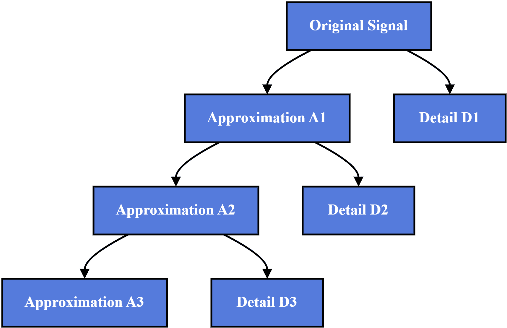
Unlike the CWT, which produces a dense, continuous time-frequency map, the DWT creates a sparse, tree-like structure. This makes it more memory-efficient and suitable for compression and denoising tasks.

3.3. Inverse Wavelet Transform

Wavelet transforms aren’t just for analysis. We can also reconstruct the original signal from its wavelet coefficients. For the CWT, the inverse is expressed as:

$x(t) = \frac{1}{C_\psi} \int_{0}^{\infty} \int_{-\infty}^{+\infty} W(a, b) \cdot \psi_{a, b}(t) \, \frac{db \, da}{a^2}$

Here:

$W(a, b)$ are the wavelet coefficients,
$\psi_{a, b}(t)$ is the scaled and shifted wavelet,
$C_\psi$ is a constant that depends on the wavelet.

This double integral reconstructs the original signal by summing all scaled and shifted versions of the wavelet, weighted by their coefficients.

4. Popular Wavelets

Wavelets come in different shapes, each suited for specific signal features and analysis goals. While the core idea is the same, localizing both time and frequency, different wavelets offer different degrees of smoothness, symmetry, and resolution trade-offs. Some offer better time resolution, while others are optimized for frequency separation or reconstruction quality. The right choice depends on what features we want to capture in the signal.

4.1. Haar Wavelet

The Haar wavelet is the simplest one. It looks like a step function and excels at detecting sudden changes in a signal:

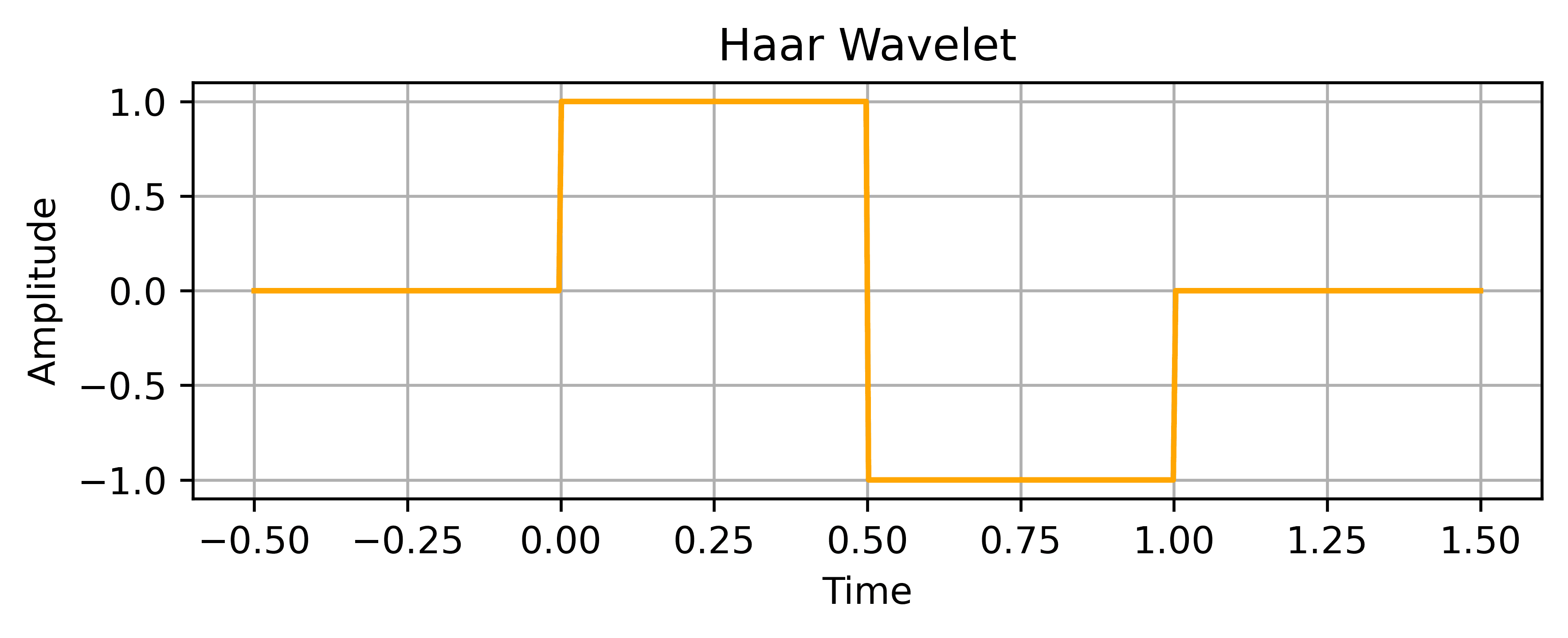Mathematically, we can represent it as:

$\psi(t) = \begin{cases} 1 & 0 \leq t < \frac{1}{2} \\ -1 & \frac{1}{2} \leq t < 1 \\ 0 & \text{otherwise} \end{cases}$

Here, $\psi(t)$ is the Haar wavelet function evaluated at time $t$ .

While it’s not smooth enough for gradual transitions, it’s fast, easy to implement, and works well in tasks like image compression and thresholding.

4.2. Daubechies Wavelets

Daubechies wavelets provide a good balance between time and frequency resolution. Each version is identified by its order, such as db4 or db8. Higher-order versions offer more smoothness and better frequency separation, but also increase computational cost.

Unlike haar, these wavelets don’t have a simple analytical form. They’re defined by a set of scaling coefficients and are generated recursively.

Let’s look at an example plot for the db4 wavelet:

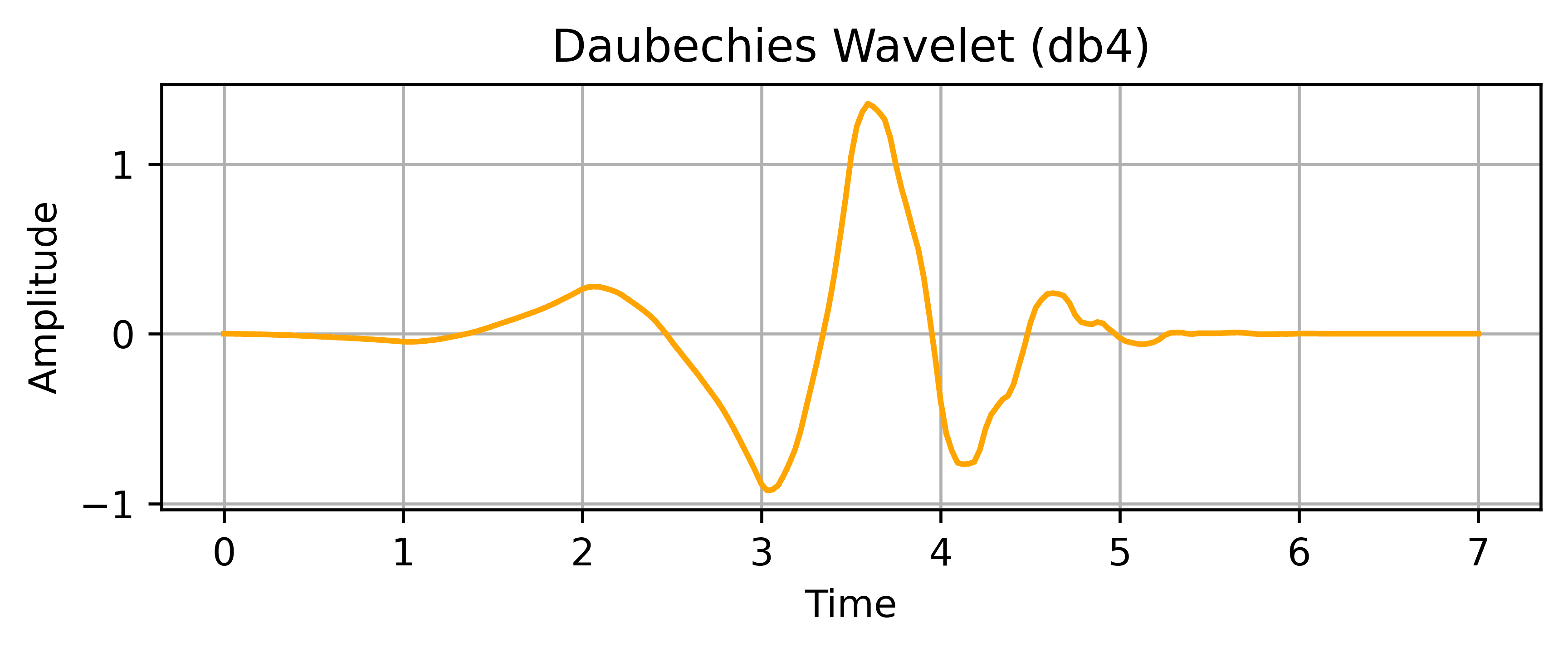
The db4 wavelet offers smoothness and time-frequency localization, making it ideal for signal denoising and compression.

4.3. Symlets

Symlets are symmetric variants of Daubechies wavelets. They’re designed to reduce phase distortion during signal reconstruction, making them a solid choice in applications like image or audio processing where symmetry matters.

Like Daubechies, Symlets don’t have a closed-form expression. They’re defined through a set of scaling filters and are available in various orders, for example, symlet 4 (sym4):

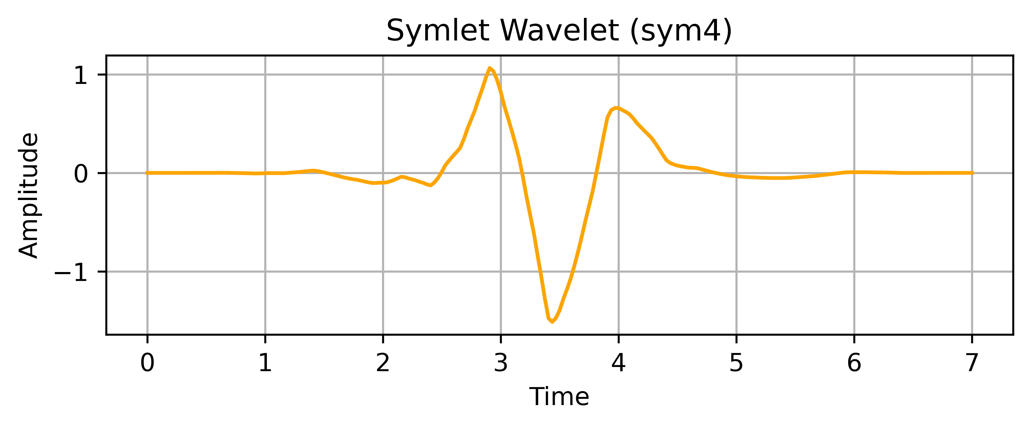
These wavelets improve symmetry while preserving smoothness, reducing phase distortion during signal reconstruction.

4.4. Morlet Wavelet

The Morlet wavelet combines a sinusoidal wave with a Gaussian window. It’s often used in the CTW to analyze oscillatory signals such as EEG or audio.

Its analytical form combines a cosine wave with exponential decay:

$\psi(t) = \cos(5t) \cdot e^{-t^2 / 2}$

In this expression, $\psi(t)$ is the Morlet wavelet function. The term $\cos(5t)$ introduces a sinusoidal oscillation, while the exponential term $e^{-t^2 / 2}$ acts as a Gaussian window that localizes the wavelet in time.

Because of its shape, it behaves similarly to Fourier-based methods but still retains time localization:

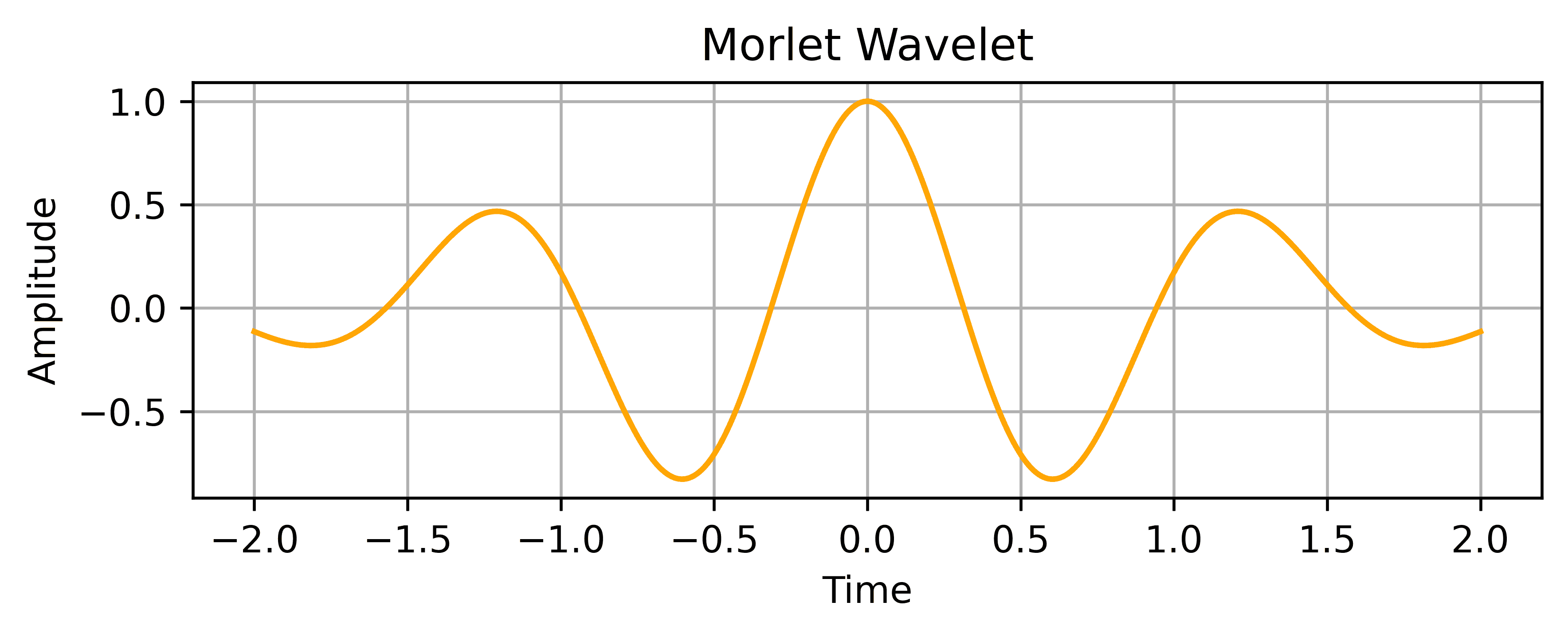
This shape makes the Morlet wavelet particularly useful for identifying frequency components localized in time.

4.5. Comparing Wavelet Functions

Different wavelets are suited to varying types of signals. We must choose the right wavelet depending on the signal’s nature and analysis goals.

Let’s look at a summary of the four wavelet types we covered and how they compare across key properties:

Wavelet	Shape	Time Localization	Frequency Localization	Symmetry	Best For
Haar	Step-like	Excellent	Poor	No	Sudden changes, edge detection
Daubechies	Smooth, compact	Good	Good	Low	General-purpose, denoising, compression
Symlet	Smooth, symmetric	Good	Good	Moderate	Signal reconstruction, phase-sensitive tasks
Morlet	Sinusoidal + Gaussian	Moderate	Excellent	Yes	Oscillatory signals, time-frequency analysis

Each wavelet has its trade-offs. Haar is ideal for quick computations and detecting sharp transitions, while Morlet offers fine-grained frequency analysis. Daubechies and Symlets are good general-purpose options, especially when smoothness and reconstruction accuracy matter.

5. Practical Examples Using PyWavelets

To see how the DTW works in practice, we’ll use the PyWavelets library in Python. This tool makes it easy to decompose and analyze signals using wavelets.

We can install the library using pip:

pip install PyWavelets

We’ll start by creating a synthetic signal that combines a slow and a fast sine wave. Then, we’ll apply the DWT to separate the low and high-frequency components.

import pywt
import numpy as np
import matplotlib.pyplot as plt

t = np.linspace(0, 1, 1024)
signal = np.sin(2 * np.pi * 5 * t) + 0.5 * np.sin(2 * np.pi * 50 * t)

approx, detail = pywt.dwt(signal, 'db4')

plt.figure(figsize=(12, 6))

plt.subplot(3, 1, 1)
plt.plot(signal)
plt.title("Original Signal")

plt.subplot(3, 1, 2)
plt.plot(approx)
plt.title("Approximation Coefficients (Low Frequencies)")

plt.subplot(3, 1, 3)
plt.plot(detail)
plt.title("Detail Coefficients (High Frequencies)")

plt.tight_layout()
plt.show()

The function pywt.dwt() takes two arguments:

signal, i.e. the input array (in our case, a composite sine wave)
and the type of wavelet to use (here, Daubechies 4 (db4)).

The function then returns approximation coefficients (approx), which capture the low-frequency part of the signal and detail coefficients (detail), which isolate the high-frequency content:

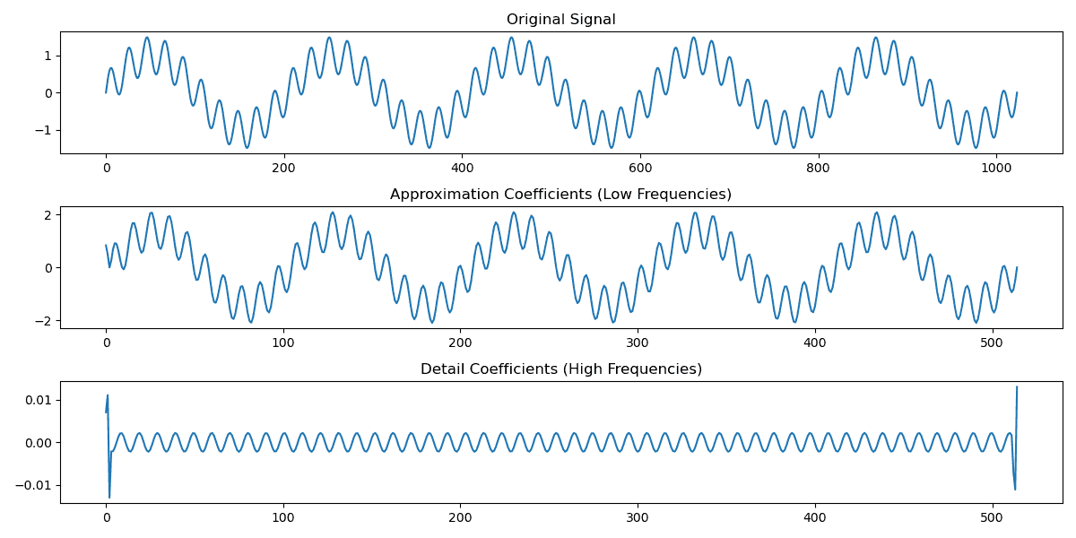
The approximation coefficients capture the slower 5 Hz oscillation, while the detail coefficients isolate the faster 50 Hz component. This decomposition shows how wavelets separate signal features by frequency and preserve their time localization

5.1. Reconstructing the Signal

After decomposing a signal with DWT, we can reconstruct it using the inverse transform. This is especially important in tasks like denoising or compression, where we might remove or modify some coefficients and then rebuild the signal.

In PyWavelets, reconstruction is as simple as calling:

reconstructed = pywt.idwt(approx, detail, 'db4')

This line combines the approximation and detail coefficients to rebuild the signal using the same wavelet. The output reconstructed is a 1D NumPy array that approximates the original signal using the inverse DWT. If we haven’t modified the coefficients, this reconstruction will closely match the original input:

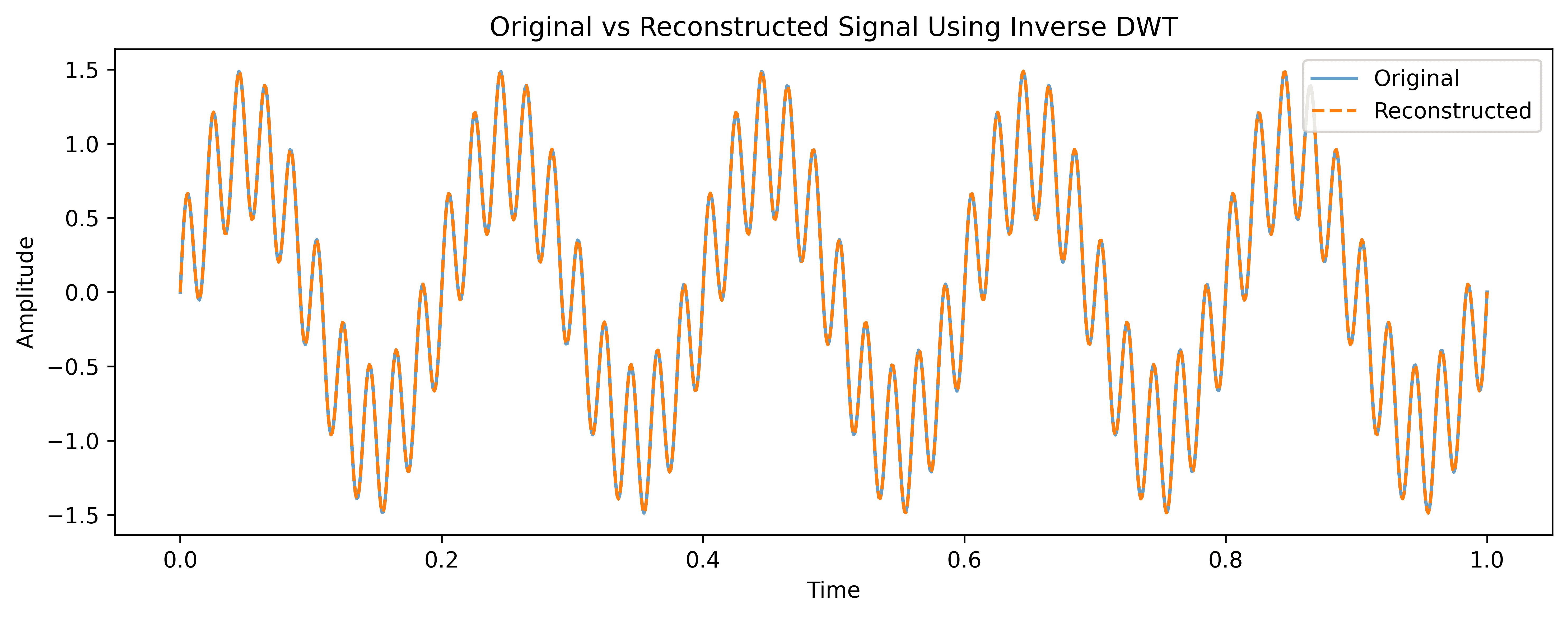
After analyzing or filtering the coefficients, we can rebuild a meaningful version of the original signal with minimal loss.

5.2. Multi-Level Decomposition

One of the main strengths of the DWT is its ability to decompose a signal across multiple levels. At each level, we apply the transform recursively to the approximation coefficients from the previous step. This gives us a hierarchical signal decomposition, from coarse trends to fine details.

In PyWavelets, we can use the wavedec() unction to perform multi-level decomposition:

coeffs = pywt.wavedec(signal, 'db4', level=3)
approx = coeffs[0]
details = coeffs[1:]

The wavedec() function returns a list of arrays. The first item, coeffs[0], represents the final approximation coefficients of the signal’s lowest frequency, smoothest version. The remaining items coeffs[1:] are the detail coefficients for each decomposition level, representing progressively higher-frequency components.

In our example, this gives us a 3-level DWT decomposition:

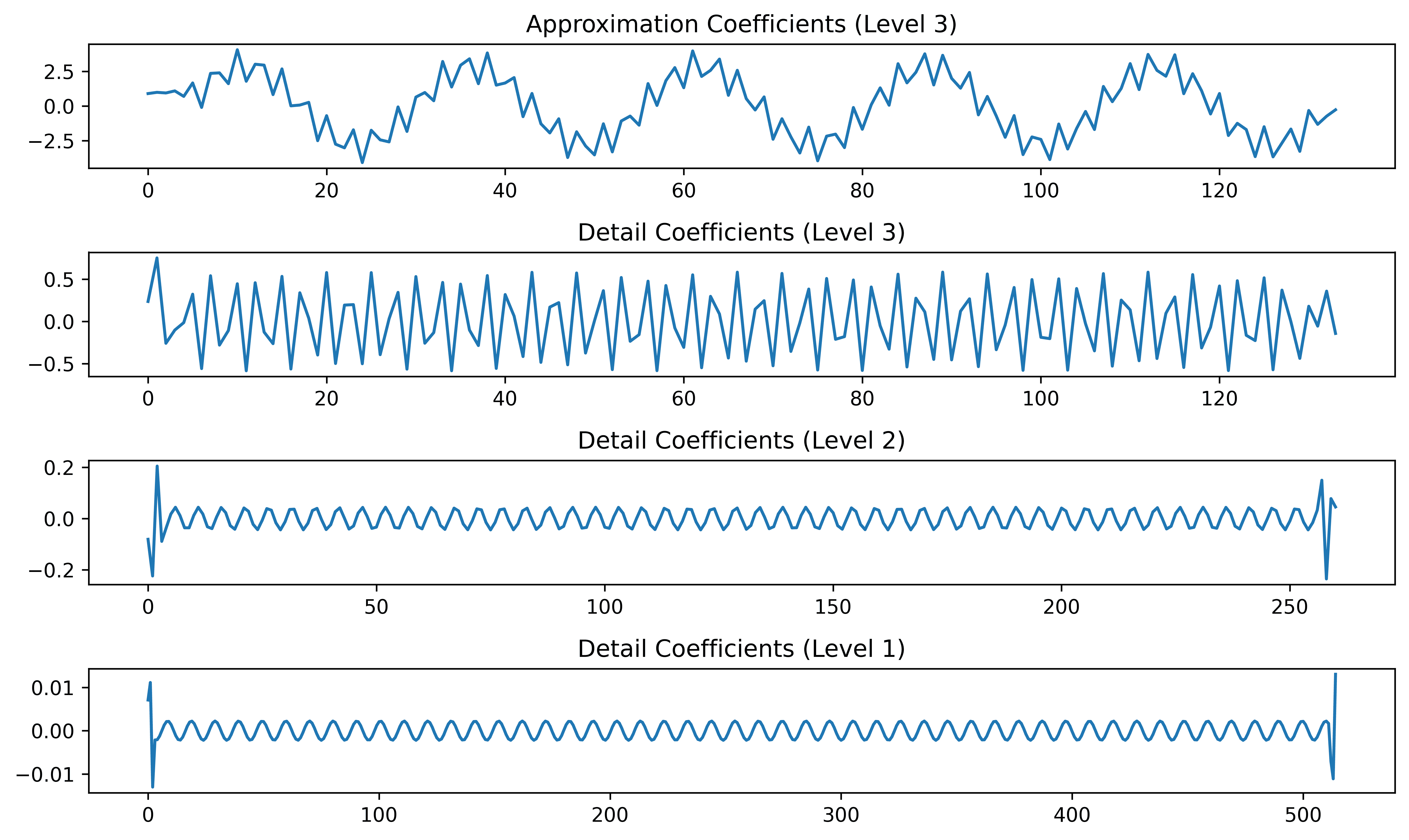
This multi-level breakdown provides a compact, layered view of the signal’s structure, which is ideal for denoising, compression, or feature extraction.

6. Applications of Wavelet Transform

The Wavelet Transform is widely used across domains thanks to its ability to capture features in both time and frequency. Here are some common use cases:

Application Area	Description
Image Compression	Used in JPEG 2000 to compress images by removing small coefficients without visible quality loss
Biomedical Signal Processing	Helps detect events like arrhythmias or epileptic spikes in ECG/EEG signals by isolating short-duration changes
Denoising	Removes noise by discarding high-frequency detail coefficients and reconstructing the clean signal
Financial Data Analysis	Captures short-term patterns, local volatility, and trend changes in stock market signals
Fault Detection	Analyzes vibration signals in mechanical systems to identify early signs of wear or failure

These examples highlight the versatility of the wavelet transform. Whether identifying subtle anomalies or optimizing data storage, wavelets provide a flexible, time-aware framework for working with real-world signals.

7. Conclusion

In this article, we explored the wavelet transform and how it helps us analyze signals at multiple resolutions.

We covered the differences between the continuous and discrete wavelet transforms, examined common wavelet types like Haar and Daubechies, and walked through a simple decomposition using PyWavelets. We also looked at real-world use cases in fields like image compression, biomedical signal analysis, and fault detection.

Unlike the Fourier Transform, which only reveals frequency content, wavelets provide a richer view that includes time and frequency information.

As a rule of thumb, we should use the CTW when we need fine-grained, time-frequency details. The DTW is usually better suited for practical tasks like compression, denoising, or real-time processing.

Core Concepts

Operating Systems

Artificial Intelligence

Graph Theory

Latex

Full Archive

About Baeldung