

Yes, we're now running our only Summer Sale. All Courses are 30% off until 20th July, 2026:
Algorithm for Online Outlier Detection in Time Series
Last updated: March 18, 2024
Learn through the super-clean Baeldung Pro experience:
>> Membership and Baeldung Pro.
No ads, dark-mode and 6 months free of IntelliJ Idea Ultimate to start with.
1. Introduction
Time series data is often subject to anomalies or outliers, which can distort the data and make it difficult to extract meaningful insights. Outliers are data points that deviate significantly from most data in a time series. Detecting and handling outliers is crucial in time series analysis, as they can distort the analysis and lead to incorrect conclusions.
In this tutorial, we’ll discuss the algorithm for online outlier detection in time series.
2. What Is Online Outlier Detection?
Online outlier detection is a method of detecting outliers in real-time. This means that the algorithm is designed to analyze data as it is received rather than analyzing pre-collected data. Online outlier detection is particularly useful in scenarios where the data is continuously generated, such as in streaming data or IoT sensors.
In contrast to batch outlier detection, which processes a fixed set of data at once, online outlier detection continuously monitors the data and identifies outliers as they occur. Indeed, traditional outlier detection methods that rely on batch processing are not well suited for online outlier detection because they require all data to be available simultaneously. Therefore, specialized algorithms and techniques have been developed to enable efficient and effective online outlier detection.
3. The Algorithm
The algorithm for online outlier detection in time series data is based on the Moving Z-Score (MZS) algorithm, a statistical method for detecting outliers in a univariate time series. The MZS algorithm computes a moving average and standard deviation of the time series data and uses them to compute a Z-score for each data point. A Z-score measures the number of standard deviations a data point is away from the mean of the time series.
The MZS algorithm is well suited for online outlier detection because it can adapt to changes in the data over time. However, the standard MZS algorithm is not suitable for detecting outliers in real time because it requires a window of data to compute the moving average and standard deviation.
In online outlier detection, we need to detect outliers as soon as they occur without waiting for a data window to accumulate.
3.1. The Modified MZS
To address the above issue, we can modify the MZS algorithm to work online using a recursive formula for computing the moving average and standard deviation. The recursive formula updates the moving average and standard deviation for each new data point without storing all the previous data points.
The modified MZS algorithm consists of the following steps:
- Compute the initial moving average and standard deviation using the first
 data points
 - For each new data point
 , compute the Z-score using the current moving average and standard deviation
 - If the Z-score exceeds a predefined threshold value, mark the data point as an outlier
- Update the moving average and standard deviation using the recursive formula
The formula for computing Z-score is as follows:
![\[Z_{\text {score }}=\left|\frac{x-MA}{SD}\right|\]](/wp-content/ql-cache/quicklatex.com-112f8c84823c873ba6b855af5f323356_l3.svg "Rendered by QuickLaTeX.com")
Also, MA (moving average) and SD (standard deviation) are calculated for a window of size of , where is the number of past data points inside the window. The formula for the moving average is as follows:
![\[MA[i]=\frac{x[i]+x[i-1]+\cdots+x[i-k+1]}{k}\]](/wp-content/ql-cache/quicklatex.com-c89a5d79e5490cbb2a9df7943aa11b6e_l3.svg "Rendered by QuickLaTeX.com")
Where:
![MA[i]](/wp-content/ql-cache/quicklatex.com-a07ff0f128eb67af9c9c5056d82cc5dc_l3.svg "Rendered by QuickLaTeX.com") is the moving average for the
is the moving average for the  window of elements.
![x[i]](/wp-content/ql-cache/quicklatex.com-9d0d86868fc69016d5aa6ff64058ae13_l3.svg "Rendered by QuickLaTeX.com") is the element of the data series.
is the element of the data series.
The formula for standard deviation is as follows:
![\[SD[i]=\sqrt{\frac{(x[i]-m)^2+(x[i-1]-m)^2+\cdots+(x[i-k+1]-m)^2}{K}}\]](/wp-content/ql-cache/quicklatex.com-0b951bd77ecc1d576cbaa0fa54f010f0_l3.svg "Rendered by QuickLaTeX.com")
Where:
![SD[i]](/wp-content/ql-cache/quicklatex.com-ccbfdf2defeee59dbe8d276dbc305792_l3.svg "Rendered by QuickLaTeX.com") is the standard deviation for the window of elements.
is the standard deviation for the window of elements. is the mean of the elements in the window.
- is the element of the data series.
When a new data point is added, the window shifts one data point to cover it and the moving average and standard deviation are updated.
The threshold value for marking a data point as an outlier can be chosen based on the desired level of sensitivity and false positive rate. A common choice for the threshold value is 3, which corresponds to a Z-score of 3 standard deviations away from the mean.
3.2. An Example
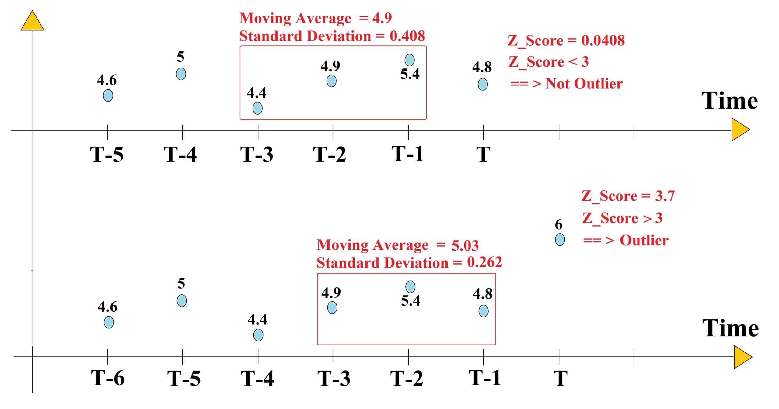
In this example, we have a time series of 5 elements, which means 5 observations or data points with the values of [4.6, 5.0, 4.4, 4.9, 5.4] have been passed. At the current time step, a new entry with the value of 4.8 is added. We want to see if this entry is an outlier or not.
First, we need to calculate the moving average and standard deviation of the window of the last elements. We consider =3, therefore we have:
![\[MovingAverage=\frac{4.4+4.9+5.4}{3}=4.9\]](/wp-content/ql-cache/quicklatex.com-d0b8e44943d23152a65eca6a058dcc3c_l3.svg "Rendered by QuickLaTeX.com")
![\[Standard Deviation=\sqrt{\frac{(4.4-4.9)^2+(4.9-4.9)^2+(5.4-4.9)^2}{3}}=0.408\]](/wp-content/ql-cache/quicklatex.com-ba0a851e8e45795dc4f2272d7950b757_l3.svg "Rendered by QuickLaTeX.com")
now we calculate the Z-score for the first new data point, 4.8:
![\[Z_{\text {score }}=\left|\frac{4.8-4.9}{0.408}\right|=0.0408\]](/wp-content/ql-cache/quicklatex.com-9ad3e0bc4f7440ccb81467c4f5468ac5_l3.svg "Rendered by QuickLaTeX.com")
We consider an entry as an outlier if the Z-score is above 3, which is not the case for the entry of 4.8 so this entry is not an outlier.
Now, we add another new entry with the value of 6 at the next time step. Let’s check to see if this entry is an outlier or not. First, we calculate the updated moving average and standard deviation.
![\[MovingAverage=\frac{4.9+5.4+4.8}{3}=5.03\]](/wp-content/ql-cache/quicklatex.com-f70a73e11f50876a52ffd1d2543bbde9_l3.svg "Rendered by QuickLaTeX.com")
![\[StandardDeviation=\sqrt{\frac{(4.9-5.03)^2+(5.4-5.03)^2+(4.8-5.03)^2}{3}}=0.262\]](/wp-content/ql-cache/quicklatex.com-c4c837a11b68bb7964a29c378cb63ee1_l3.svg "Rendered by QuickLaTeX.com")
now we calculate the Z-score for the next new data point, 6:
![\[Z_{\text {score }}=\left|\frac{6-5.03}{0.262}\right|=3.7\]](/wp-content/ql-cache/quicklatex.com-55c98e97ccf1dd3fae9a1dcec435e18c_l3.svg "Rendered by QuickLaTeX.com")
Since the Z-score is above 3, we can call the new entry an outlier. The below figure shows the process for these two new entries:
3.3. An Alternative for Standard Deviation in MZS
Median Absolute Deviation (MAD) is an alternative to the standard deviation for calculating the dispersion of a dataset. Instead of using the standard deviation, which is sensitive to outliers, MZS uses the MAD in its calculation. MAD is a measure of the variability of a dataset based on the median of the absolute deviations from the median of the data.
The formula for MZS using MAD instead of standard deviation is as follows:
![\[Z_{\text {score }}=\left|\frac{0.6745*(x-median(x))}{MAD}\right|\]](/wp-content/ql-cache/quicklatex.com-ee0a849888b8cf0532416696cb022e0a_l3.svg "Rendered by QuickLaTeX.com")
Where:
- is a data point.
- median(x) is the median of the window.
- MAD is calculated as:
![\[MAD = median(|x - median(x)|)\]](/wp-content/ql-cache/quicklatex.com-1cc621cd4dcd25e5be7b2e76790ba863_l3.svg "Rendered by QuickLaTeX.com")
The factor 0.6745 is a scaling factor that makes MZS comparable to the standard deviation for normally distributed data.
To see how it works, we’ll calculate the MZS by MAD for the new entry 4.8 in the previous example. The median of the window [4.4, 4.9, 5.4] is 4.9. To calculate the MAD, we first calculate the absolute deviations from the median:
![\[|4.4 - 4.9| = 0.5\]](/wp-content/ql-cache/quicklatex.com-75cd6cc0cfae681bbf8c4bf16cf5977d_l3.svg "Rendered by QuickLaTeX.com")
![\[|4.9 - 4.9| = 0\]](/wp-content/ql-cache/quicklatex.com-98cc4bfec3f7b257be0bf0507c02337e_l3.svg "Rendered by QuickLaTeX.com")
![\[|5.4 - 4.9| = 0.5\]](/wp-content/ql-cache/quicklatex.com-589e092b09fa639c1e48d031418ef13a_l3.svg "Rendered by QuickLaTeX.com")
Then, we take the median of these absolute deviations:
![\[MAD = median(0.5, 0, 0.5) = 0.5\]](/wp-content/ql-cache/quicklatex.com-11d3e238eda912dcf57e9b5e57438147_l3.svg "Rendered by QuickLaTeX.com")
Now we can calculate the MZS score for the new entry 4.8:
![\[Z_{\text {score }}=\left|\frac{0.6745*(4.8-4.9)}{0.5}\right|=0.2698\]](/wp-content/ql-cache/quicklatex.com-22c3580a88e2e8ff1936d7522d1a147f_l3.svg "Rendered by QuickLaTeX.com")
Which is under 3 and indicates that the new entry is not an outlier.
Using MAD instead of standard deviation in MZS makes it more robust to outliers since MAD is less affected by extreme values than standard deviation. MZS can detect outliers by comparing the absolute value of MZS to a threshold value. Data points with MZS above the threshold are considered outliers.
4. The Pros and Cons
The pros and cons of the MZS algorithm for online outlier detection are as follows:
| Pros | Cons |
|---|---|
| Simple and easy to implement | Limited adaptability to non-stationary data streams |
| Robust to outliers | Susceptibility to false positives and false negatives |
| Applicable to a wide range of data types | Difficulty in detecting context-dependent outliers |
5. Alternative Algorithms
Several algorithms can be used for online outlier detection. Here we present three algorithms that tackle one limitation of MZS, as described in the previous section.
The choice of algorithm depends on the application’s specific requirements such as the data characteristics, the expected rate of outliers, and the desired trade-off between false positives and false negatives.
5.1. Dynamic Z-Score (DZS)
To address the limitation of MZS’s adaptability to non-stationary data streams, the DZS algorithm was proposed. The DZS algorithm adapts the threshold value of the outlier detection based on the statistical properties of the data stream. The threshold value is adjusted according to the variation of the MAD of the data stream over time. This approach enables the DZS algorithm to adapt to changes in the statistical properties of the data stream and to detect outliers more accurately in non-stationary data streams.
5.2. Robust Mahalanobis Distance (RMD)
To address the limitation of MZS’s susceptibility to false positives and false negatives, the RMD algorithm was proposed. The RMD algorithm uses a robust measure of distance instead of the modified Z-score to detect outliers. The Mahalanobis distance is a measure of the distance between a data point and the centre of a distribution, considering the covariance matrix of the data. The RMD algorithm uses a robust covariance matrix estimator, such as the Minimum Covariance Determinant (MCD) or the Sparse Covariance Estimation (SCE), to calculate the Mahalanobis distance. This approach enables the RMD algorithm to handle skewed distributions, heavy-tailed data, and outliers more effectively than the MZS algorithm.
5.3. Context-Based Outlier Detection (CBOD)
To address the difficulty of detecting context-dependent outliers, the CBOD algorithm was proposed. The CBOD algorithm uses a clustering approach to group similar data points based on their contextual attributes. The algorithm then applies outlier detection within each cluster separately, taking into account the context-specific characteristics of the data. This approach enables the CBOD algorithm to detect context-dependent outliers more accurately than the MZS algorithm.
6. Conclusion
In this article, we examined the MZS as a popular algorithm for online outlier detection, introduced its pros and cons, and reviewed other alternative algorithms.