Using a Hard Margin vs. Soft Margin in SVM | Baeldung on Computer Science

1. Overview

Support Vector Machines are a powerful machine learning method to do classification and regression. When we want to apply it to solve a problem, the choice of a margin type is a critical one. In this tutorial, we’ll zoom in on the difference between using a hard margin and a soft margin in SVM.

2. The Role of Margin in SVMs

Let’s start with a set of data points that we want to classify into two groups. We can consider two cases for these data: either they are linearly separable, or the separating hyperplane is non-linear. When the data is linearly separable, and we don’t want to have any misclassifications, we use SVM with a hard margin. However, when a linear boundary is not feasible, or we want to allow some misclassifications in the hope of achieving better generality, we can opt for a soft margin for our classifier.

2.1. SVM with a Hard Margin

Let’s assume that the hyperplane separating our two classes is defined as $\pmb{w^T x} + b = 0$ :

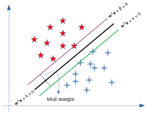
Then, we can define the margin by two parallel hyperplanes:

$\pmb{w^T x} + \alpha = 0,$

$\pmb{w^T x} + \beta = 0$

They are the green and purple lines in the above figure. Without allowing any misclassifications in the hard margin SVM, we want to maximize the distance between the two hyperplanes. To find this distance, we can use the formula for the distance of a point from a plane. So the distance of the blue points and the red point from the black line would respectively be:

$\frac {|\pmb{w^T x} + \alpha|}{||\pmb{w}||} \hspace{2mm} \textnormal{and} \hspace{2mm} \frac {|\pmb{w^T x} + \beta|}{||\pmb{w}||}$

As a result, the total margin would become:

$\frac{|\alpha - \beta|}{||\pmb{w}||}$

We want to maximize this margin. Without the loss of generality, we can consider $\alpha = b + 1$ and $\beta = b - 1$ . Subsequently, the problem would be to maximize $\frac{2}{||\pmb{w}||}$ or minimize $\frac{||\pmb{w}||}{2}$ . To make the problem easier when taking the gradients, we’ll, instead, word with its squared form:

$\mathop{\textnormal{min}}_{\pmb{w}, b} \hspace{2mm} \frac{1}{2} ||\pmb{w}||^2 \equiv \mathop{\textnormal{min}}_{\pmb{w}, b} \hspace{2mm} \frac{1}{2} \pmb{w}^T \pmb{w}$

This optimization comes with some constraints. Let’s assume that the labels for our classes are {-1, +1}. When classifying the data points, we want the points belonging to positives classes to be greater than $+1$ , meaning $\pmb{w}^T \pmb{x} + b \geq 1$ , and the points belonging to the negative classes to be less than $-1$ , i.e. $\pmb{w}^T \pmb{x} + b \leq -1$ .

We can combine these two constraints and express them as: $y_i (\pmb{w}^T \pmb{x}_i + b) \geq 1$ . Therefore our optimization problem would become:

$\mathop{\textnormal{min}}_{\pmb{w}, b} \hspace{1mm} \frac{1}{2} \pmb{w}^T \pmb{w}$

$\textnormal{\textbf{s.t.}} \hspace{3mm} y_i (\pmb{w}^T \pmb{x}_i + b) \geq 1$

This optimization is called the primal problem and is guaranteed to have a global minimum. We can solve this by introducing Lagrange multipliers ( $\alpha_i$ ) and converting it to the dual problem:

$L(\pmb{w}, b, \alpha_i) = \frac{1}{2} \pmb{w^T w} - \sum_{i=1}^{n} \alpha_i (y_i (\pmb{w^T x}_i + b) -1)$

This is called the Lagrangian function of the SVM which is differentiable with respect to $\pmb{w}$ and b.

$\nabla_{\pmb{w}} L(\pmb{w}, b, \alpha) = 0 \Rightarrow \pmb{w} = \sum_{i=1}^{n} \alpha_i y_i x_i$

$\nabla_{b} L(\pmb{w}, b, \alpha) = 0 \Rightarrow \sum_{i=1}^{n} \alpha_i y_i =0$

By substituting them in the second term of the Lagrangian function, we’ll get the dual problem of SVM:

$\mathop{\textnormal{max}}_{\pmb{\alpha}} \hspace{1mm} -\frac{1}{2} \sum_{i=1}^{n} \sum_{j=1}^{n} \alpha_i \alpha_j y_i y_j x_i^T x_j + \sum_{i=1}^{n} \alpha_i$

$\textbf{s.t.} \hspace{3mm} \sum_{i=1}^{n} \alpha_i y_i = 0$

The dual problem is easier to solve since it has only the Lagrange multipliers. Also, the fact that the dual problem depends on the inner products of the training data comes in handy when extending linear SVM to learn non-linear boundaries.

2.2. SVM with a Soft Margin

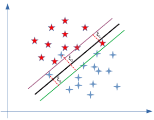
The soft margin SVM follows a somewhat similar optimization procedure with a couple of differences. First, in this scenario, we allow misclassifications to happen. So we’ll need to minimize the misclassification error, which means that we’ll have to deal with one more constraint. Second, to minimize the error, we should define a loss function. A common loss function used for soft margin is the hinge loss.

$\textnormal{max} \{0, 1 - y_i (\pmb{w}^T \pmb{x}_i + b) \}$

The loss of a misclassified point is called a slack variable and is added to the primal problem that we had for hard margin SVM. So the primal problem for the soft margin becomes:

$\textnormal{min} \hspace{1mm} \frac{1}{2} ||\pmb{w}||^2 + C \sum_{i=1}^{n} \zeta_i$

$\textnormal{\textbf{s.t.}} \hspace{3mm} y_i (\pmb{w}^T \pmb{x}_i + b) \geq 1 - \zeta_i \hspace{4mm} \forall i=1, ..., n, \hspace{1mm} \zeta_i \geq 0$

A new regularization parameter $C$ controls the trade-off between maximizing the margin and minimizing the loss. As you can see, the difference between the primal problem and the one for the hard margin is the addition of slack variables. The new slack variables ( $\zeta_i$ in the figure below) add flexibility for misclassifications of the model:

Finally, we can also compare the dual problems:

$\textnormal{max} \hspace{1mm} -\frac{1}{2} \sum_{i=1}^{n} \sum_{j=1}^{n} \alpha_i \alpha_j y_i y_j x_i^T x_j + \sum_{i=1}^{n} \alpha_i$

$\textbf{s.t.} \hspace{3mm} \sum_{i=1}^{n} \alpha_i y_i = 0, \hspace{2mm} 0 \leq \alpha_i \leq C$

As you can see, in the dual form, the difference is only the upper bound applied to the Lagrange multipliers.

3. Hard Margin vs. Soft Margin

The difference between a hard margin and a soft margin in SVMs lies in the separability of the data. If our data is linearly separable, we go for a hard margin. However, if this is not the case, it won’t be feasible to do that. In the presence of the data points that make it impossible to find a linear classifier, we would have to be more lenient and let some of the data points be misclassified. In this case, a soft margin SVM is appropriate.

Sometimes, the data is linearly separable, but the margin is so small that the model becomes prone to overfitting or being too sensitive to outliers. Also, in this case, we can opt for a larger margin by using soft margin SVM in order to help the model generalize better.

4. Conclusion

In this tutorial, we focused on clarifying the difference between a hard margin SVM and a soft margin SVM.

Full Archive

About Baeldung

Core Concepts

Operating Systems

Artificial Intelligence

Graph Theory

Latex