Computer Vision: Stereo 3D Vision | Baeldung on Computer Science

1. Introduction

In this tutorial, we’ll talk about stereo vision, a type of machine vision that uses two or more cameras to produce a full-field-of-view 3D measurement.

2. What Is Stereo (3D) Vision?

Computer stereo vision is the extraction of 3D information from 2D images, such as those produced by a CCD camera. It compares data from multiple perspectives and combines the relative positions of things in each view. As such, we use stereo vision in applications like advanced driver assistance systems and robot navigation.

It’s similar to how human vision works. Our brains’ simultaneous integration of the images from both of our eyes results in 3D vision:

Although each eye produces only a two-dimensional image, the human brain can perceive depth when combining both views and recognizing their differences. We call this ability stereo vision.

3. Perceiving Depth

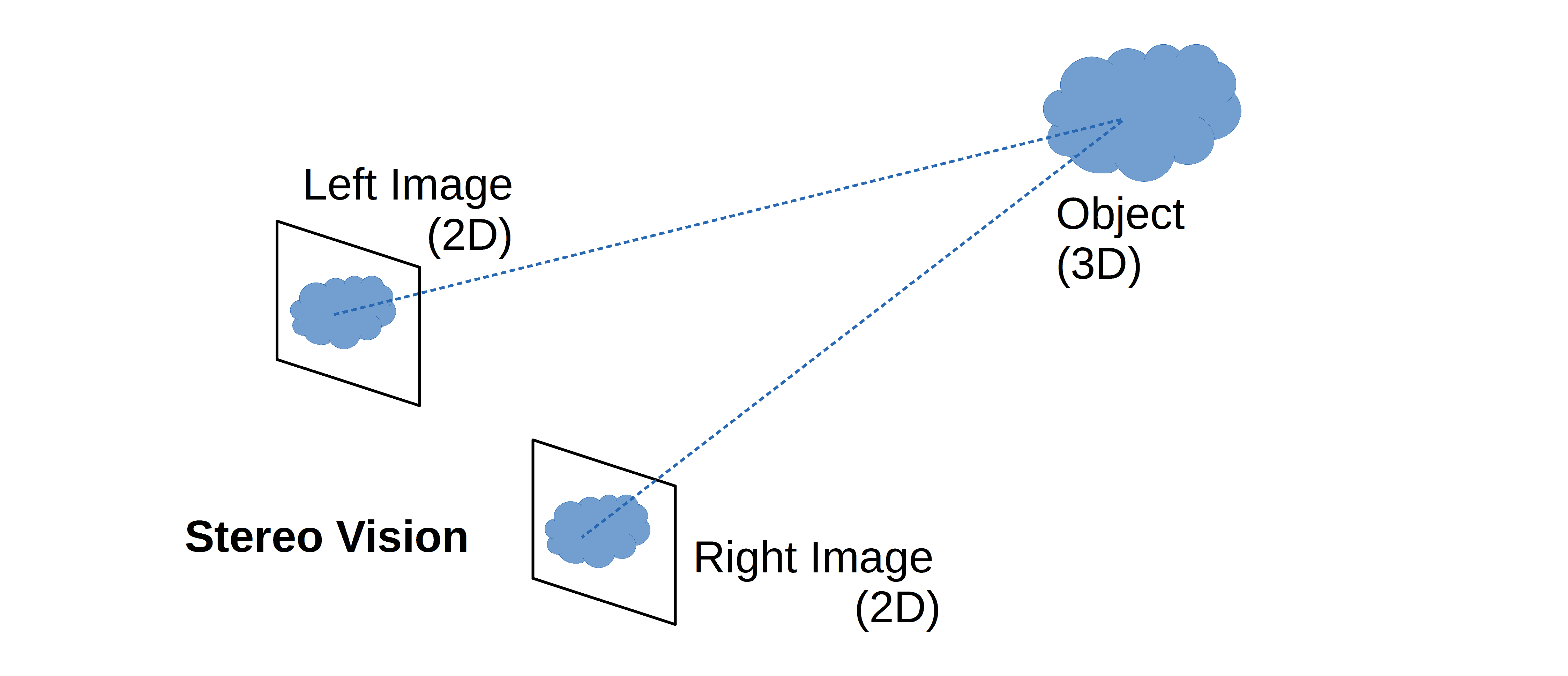
Let’s suppose there are left and right cameras, both producing a 2D image of a scene. Let S be a point on a real-world (3D) object in the scene:

To determine the depth of S in the composite 3D image, we first find two pixels L and R in the left and right 2D images that correspond to it. We can assume that we know the relative positioning of the two cameras. The computing system estimates the depth d by triangulation using the prior knowledge of the relative distance between the cameras.

The human brain works the same way. Its ability to perceive depth and 3D forms is known as stereopsis.

4. How Computer Systems Achieve Stereo Vision

We need to estimate each point’s depth to produce a 3D image from two-dimensional ones. From there, we can determine the points’ relative depths and get a depth map:

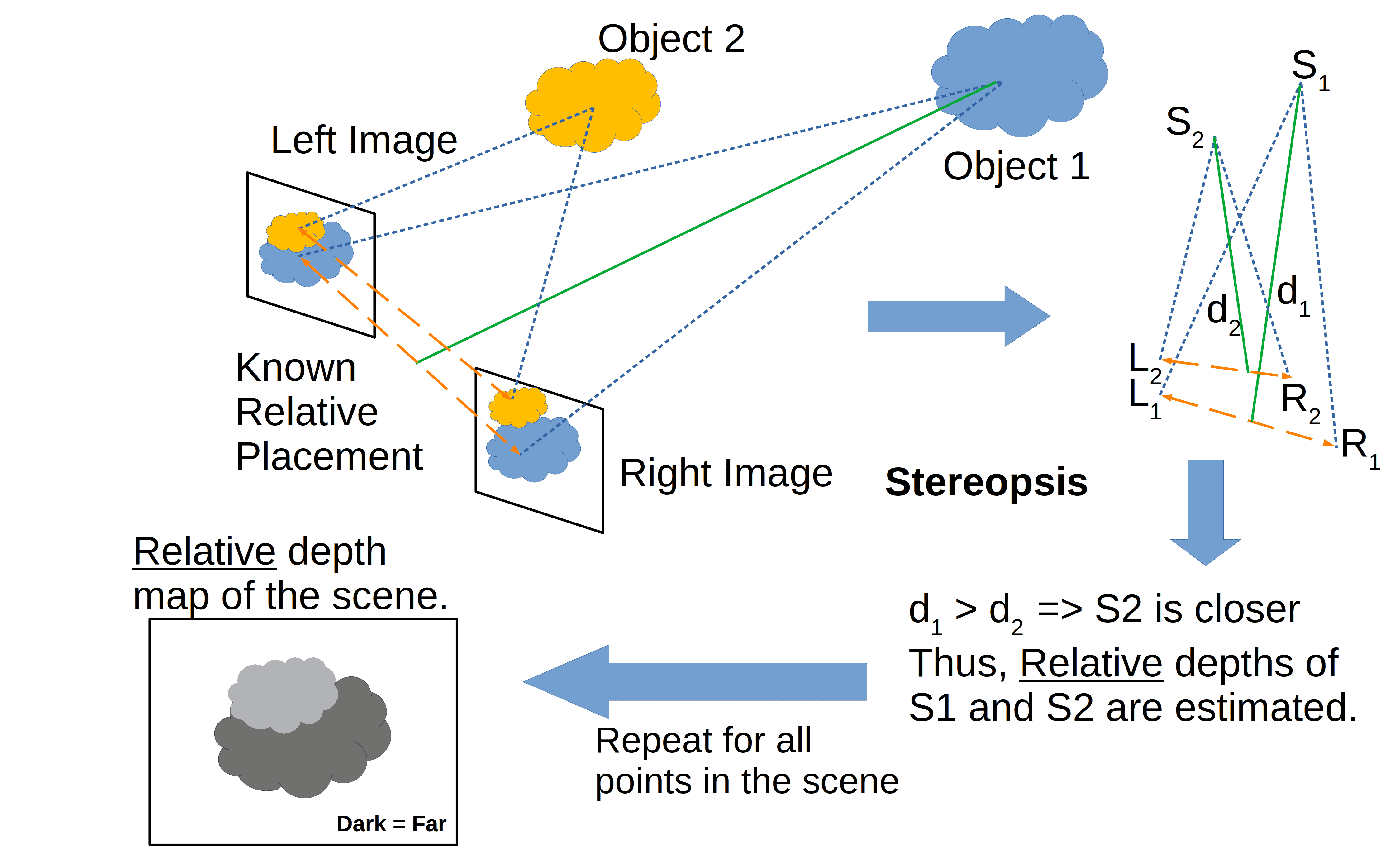
A depth map is an image (or image channel) that contains the data on the separation between the surfaces of scene objects from a viewpoint. This is a common way to represent scene depths in 3D computer graphics and computer vision. We can see an example of a depth map in the bottom left corner of the above image.

5. The Geometrical Basis of Stereo Vision

Epipolar geometry is the geometry of stereo vision. There are a variety of geometric relationships between the 3D points and their projections onto the 2D images. These relationships have been developed for the pinhole camera model. We assume that we can represent normal using these relationships.

A 3D item is projected into a 2D (planar) projective space when captured (projected) in an image. The issue with this so-called “planar projection” is that it causes the loss of depth.

The disparity between the two stereo pictures is the apparent motion of things. If we close one eye and open it quickly while keeping the other closed, we’ll observe that objects near us move quite a bit, whereas those farther away move barely at all. We refer to this phenomenon as “discrepancy.”

5.1. The Direction Vector

In epipolar geometry, a direction vector is a vector in three dimensions emanating from a pixel in the image:

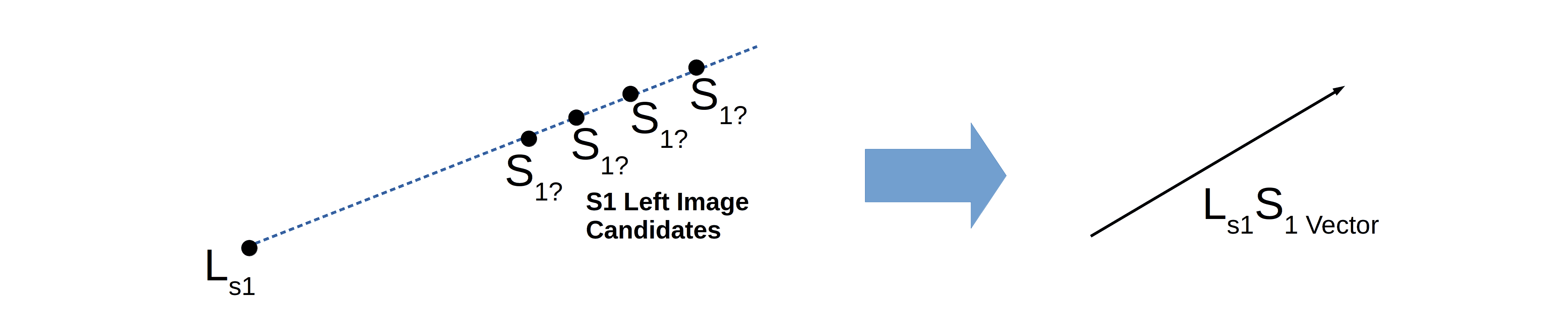
The direction vector, as the name suggests, is the direction from where the light ray arrives at the pixel sensor. This line thus carries all the 3D points that could be candidate sources for the 2D pixels in the image. In the above figure, the direction vector $L_{s1}S_1$ originates from the point $L_{s1}$ , which is the “left” 2D pixel corresponding to the 3D point $S_1$ in the scene.

5.2. Direction Vector Intersection

Direction vectors for a 3D point in the scene will cast corresponding 2D points in the images taken from different views. A stereo pair of images will thus have direction vectors emanating from the 2D pixels representing a common 3D point in the 3D scene. All points on a direction vector are candidate sources. Since two vectors can intersect at only one unique point, we take the intersection point as the source:

Epipolar Geometry Direction Vector Intersection 2

In the above figure, the direction vectors from the left and right images ( $L_{s1}S_1$ and $R_{s1}S_1$ , respectively) intersect at the single source $S_1$ . This 3D source point in the scene is the point from where light rays cast image pixels $L_{s1}$ and $R_{s1}$ in the left and right images.

5.3. Depth Calculation

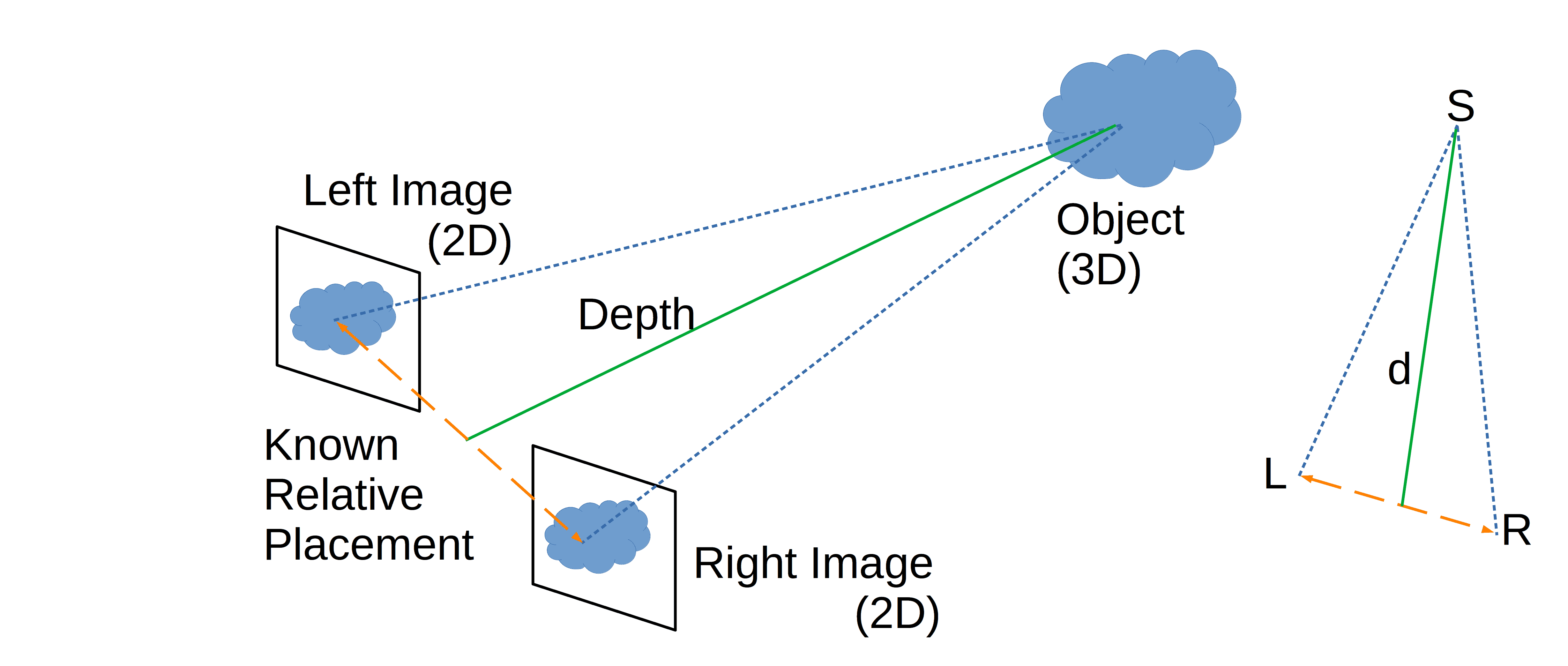
We assume that we know the distance between cameras and that it’s very small compared to the distance between the object and the cameras. Under that assumption, we can determine the location of the 3D point in space by triangulation. The depth is a perpendicular cast on the line joining the two cameras:

Epipolar Geometry Direction Vector Triangulation 1

The above image shows the actual depth $d_{s1}$ for the point from the line joining the two cameras. Let’s note that the angle between the line $d_{s1}$ and the line $L_{s1}R_{s1}$ is not exactly 90 degrees. In reality, however, the distance $L_{s1}R_{s1}$ is very small compared to $d_{s1}$ . This results in the angle between the line $d_{s1}$ and the line $L_{s1}R_{s1}$ being approximately 90 degrees. Since we determined the location of $S_1$ by triangulation, and we know the relative distance $L_{s1}R_{s1}$ , we can calculate the depth $d_{s1}$ using the Pythagorean theorem:

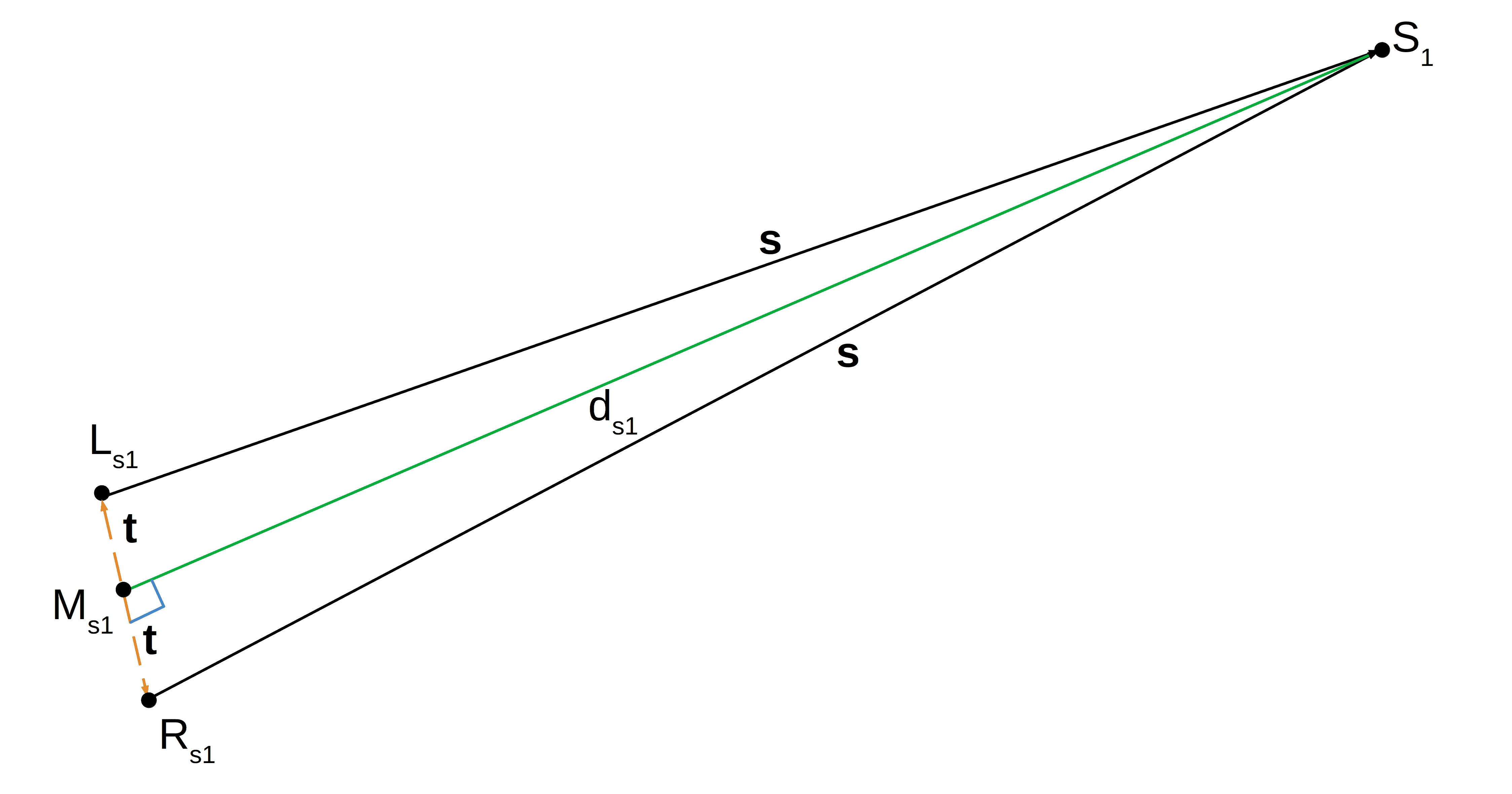
Since s is very large compared to t, the angle $\angle S_1 M_{s1 }R_{s1}$ approaches $90^{\circ}$ . Lengths $L_{s1}M_{s1}$ and $M_{s1}R_{s1}$ are almost the same (denoted by t). Also, lengths $L_{s1}S_1$ and $R_{s1}S_1$ are almost the same (denoted by s). Applying the Pythagorean theorem, we get $s^2 = {d_{s1}}^2 + t^2$ . Solving for the depth of point $S_1$ we get:

$d_{s1} = \sqrt{s^2 - t^2}$

Since s is very large compared to t, the depth $d_{s1}$ is close to $s$ .

6. Key Concepts for Mathematical Implementation of Stereo Vision

Triangulation and disparity maps are tools we need for computer stereo vision. At the pixel level, we use triangulation to identify a point in 3D space from the left and right pixel points in a pair of stereo images. We use a disparity map for large images with millions of pixel points.

6.1. Triangulation in Computer Vision

Triangulation in computer vision is the process of identifying a point in 3D space from its projections onto two or more images. The camera matrices represent the parameters of the camera projection function from 3D scene to 2D image space. The inputs for the triangulation method are the homogeneous coordinates of the detected image points ( $L_{s1}$ and $R_{s1}$ ) and the camera matrices for the left and right cameras.

The output of the triangulation method is a 3D point in the homogeneous representation. The triangulation method just represents a computation in an abstract form; in reality, the calculation may be quite complex. Some triangulation techniques require decomposition into a series of computational stages, such as SVD or determining the roots of a polynomial. Closed-form continuous functions are another set of triangulation techniques.

Another class of triangulation techniques uses iterative parameter estimation. This implies that the various methods may differ in terms of computation time and the procedures’ complexity. The mid-point method, direct linear transformation, and essential matrix are common mathematical tools we use for triangulation.

6.2. Disparity-Map

The disparity is the horizontal displacement of a point’s projections between the left and the right image. In contrast, depth refers to the depth coordinate of a point located in the real 3D world.

To create a disparity map from a pair of stereo images, we must first match each pixel in the left image with its corresponding pixel in the right image. We calculate the distance between each matching pair of pixels. We use this distance data to generate an intensity image, called the disparity map.

To compute the disparity map, we must solve the so-called correspondence problem. This job aims to identify the stereo picture pairs of pixels that are projections of the same actual physical point in space. The correction of the stereo pictures can lead to a significant simplification of the issue. The matching points will be on the same horizontal line following this transformation, transforming the 2D stereo correspondence problem into a 1D problem. This is how we break the “Curse of Dimensionality“.

The Block Matching algorithm is a fundamental method for identifying related pixels. A comparison between a small window encircling a point in the first image and several small blocks arranged along a single horizontal line in the second image forms the basis for the block-matching algorithm. The two primary similarity measures used for window matching are the Sum of Absolute Differences (SAD) and the Sum of Squared Differences (SSD).

The discrepancy has an inverse relationship with depth. We triangulate the disparity map, converting it into a depth map using the cameras’ geometric configuration as input.

7. Conclusion

In this article, we learned how contemporary computers implement the stereo vision. We derive disparity maps from pairs of stereo pictures. Then, we calculate the distance between each matching pair of pixels in the disparity map. Knowing the two cameras’ precise locations allows for the depth map’s computation.

Full Archive

About Baeldung

Core Concepts

Operating Systems

Artificial Intelligence

Graph Theory

Latex