Learn through the super-clean Baeldung Pro experience:
>> Membership and Baeldung Pro.
No ads, dark-mode and 6 months free of IntelliJ Idea Ultimate to start with.
Last updated: February 28, 2025

Learn through the super-clean Baeldung Pro experience:
>> Membership and Baeldung Pro.
No ads, dark-mode and 6 months free of IntelliJ Idea Ultimate to start with.
In this tutorial, we’ll provide a quick introduction to the sparse coding neural networks concept.
Sparse coding, in simple words, is a machine learning approach in which a dictionary of basis functions is learned and then used to represent input as a linear combination of a minimal number of these basis functions.
Moreover, sparse coding seeks a compact, efficient data representation, which may be utilized for tasks such as denoising, compression, and classification.
In the case of sparse coding, the data is first translated into a high-dimensional feature space, where the basis functions are then employed to represent the data as a linear combination of a limited number of these basis functions.
Subject to a sparsity constraint that promotes the coefficients to be zero or nearly zero, the coefficients of linear combinations are selected to reduce the reconstruction error between the original data and the representation. So, with most of the coefficients being zero or almost zero, this sparsity constraint pushes the final representation to be a linear combination of the basis functions.
In this way, sparse coding, as previously noted, seeks to discover a usable sparse representation of any given data. Then, a sparse code will be used to encode data:
Sparse coding techniques aim to meet the following two constraints simultaneously:
 for a given data
  (as a vector) using an encoder matrix
  using a decoder matrix for each representation is given as a vector
 We assume our data satisfies the following equation:
(1) 
 to generate a dictionary of basis functions and the generated dictionary ()
The general form of the target function to optimize the dictionary learning process may be mathematically represented as follows:
(2) 
In the previous equation,  is a constant;
  denotes the dimensionality of data; and
  means the k-given vector of the data. Furthermore,
  is the sparse representation of ; is the decoder matrix (dictionary); and the coefficient of sparsity is
  .
.
The min expression in the general form gives the impression that we are attempting to nest two optimization issues. We can think of this as two separate optimization issues fighting to get the optimal compromise:
to reduce the input’s loss during the reconstruction process of the sparse representation h. Said, we are trying to solve a problem (in this case, reconstruction) while utilizing the fewest resources feasible to store our data
The following algorithm performs sparse coding by iteratively updating the coefficients for each sample in the dataset, using the residuals from the previous iteration to update the coefficients for the current iteration. The sparsity constraint is enforced by setting the coefficients to zero or close to zero if they fall below a certain threshold.
algorithm SparseCodingLearningProcess(X, N, D):
    // INPUT
    //    X = the dataset with N samples and D features
    //    K = dictionary size
    //    λ = sparsity constraint
    //    max_iter = maximum number of iterations
    // OUTPUT
    //    D = the dictionary of basis functions

    // Initialize the dictionary of basis functions
    D <- a random K x D matrix

    while there is an x in X:
        r <- x

        while i < max_iter:
            while there is d in D:
                D` <- apply Eq.(2)

        D_x <- D`

return DFrom a biological perspective, sparse code follows the more all-encompassing idea of neural code. Consider the case when you have binary neurons. So, basically:
Now that we know what a neural code is, we can speculate on what it may be like. Then, data will be encoded using a sparse code while taking into consideration the following scenarios:
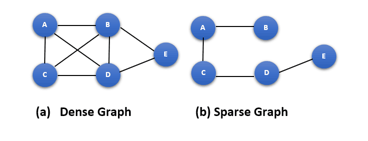
The figure next shows an example of how a dense neural network graph is transformed into a sparse neural network graph:
Brain imaging, natural language processing, and image and sound processing all use sparse coding. Also, sparse coding has been employed in leading-edge systems in several areas and has shown to be very successful at capturing the structure of complicated data.
Resources for the implementation of sparse coding are available in several Python modules. A well-known toolkit called Scikit-learn offers a light coding module with methods for creating a dictionary of basis functions and sparsely combining these basis functions to encode data.
In short, sparse coding is a powerful machine learning technique that allows us to find compact, efficient representations of complex data. It has been widely applied to various applications such as brain imaging, natural language processing, and image and sound processing and achieved promising results.