

Learn through the super-clean Baeldung Pro experience:
>> Membership and Baeldung Pro.
No ads, dark-mode and 6 months free of IntelliJ Idea Ultimate to start with.
Learn through the super-clean Baeldung Pro experience:
>> Membership and Baeldung Pro.
No ads, dark-mode and 6 months free of IntelliJ Idea Ultimate to start with.
In this tutorial, we’ll talk about the Slime Mould Algorithm and its implementation through Python code.
The Slime Mould Algorithm (SMA) mimics the problem-solving behavior of slime mould, proving effective in tasks like pathfinding and network optimization. Utilizing agents representing mould expansion toward food sources, the algorithm combines competition and cooperation to form optimal networks. This iterative process, repeated multiple times, yields solutions for various problems.
The Slime Mould Algorithm (SMA) has found application in diverse optimization problems, encompassing areas such as network design, facility location, and scheduling. It has demonstrated its effectiveness and efficiency as an algorithm in addressing these various problem domains.
Phase-based learning is a crucial mechanism in the Slime Mould Algorithm, enabling it to effectively balance exploration and exploitation, leading to robust and efficient optimization results. It refers to its cyclic behavior through two distinct phases:
This phase represents exploration. The algorithm extends tendrils outwards from its current position, mimicking the slime mould’s exploration of its environment. These tendrils represent candidate solutions, and their movement is guided by a combination of fitness values (attractiveness of food sources) and random exploration.
This randomness helps in avoiding premature convergence and allows the algorithm to discover promising regions in the search space.
This phase signifies exploitation. Once a promising candidate solution (food source) is identified, the algorithm focuses on refining its quality. The tendrils surrounding the food source thicken and contract inwards, similar to the slime mould’s veins thickening around a discovered food source.
This contraction improves the solution’s accuracy and leads to further exploitation of the promising region.
We initiate the algorithm construction process, consisting of two primary phases: the approach (search) food phase and the wrap (exploit) food phase, respectively. The algorithm will cyclically alternate between these two phases.
Before commencing the search, it’s imperative to initialize the algorithm. Despite the slime mould being a single entity in one sense, it can act at various locations along with itself. Consequently, we treat it as a fixed number of distinct entities or locations.
To begin, we initialize  locations to represent the slime mould. Subsequently, for each of these locations, we calculate the fitness of the slime mould.
The detection of food by the slime mould occurs through the perception of its odor in the air. We express this process of capturing the approaching food through odor with the following equation:
(1) 
In this context, two randomly chosen locations of our mould are denoted as  and
and  . Additionally, we use
  to represent the best individual discovered thus far. The initial condition involves the exploration of food by utilizing the information from the best-discovered location and blending it with two randomly selected locations. The subsequent condition directs the slime mould to exploit the food source available in its local vicinity.
(2) 
(3) 
With  defined above, we now define
  as a random sample from the range
 ![[−a, a]](/wp-content/ql-cache/quicklatex.com-4214a4ed5ea7a6ca08a539605208edcf_l3.svg "Rendered by QuickLaTeX.com") . We also define
. We also define  as a random variable chosen from the linearly decreasing range
 ![[-(1-\frac{i}{max_it}),(1-\frac{i}{max_it})]](/wp-content/ql-cache/quicklatex.com-47b544402ab52409898158ab3d60a3dc_l3.svg "Rendered by QuickLaTeX.com") :
:
(4) 
 is the weight parameter. The condition is that
  is in the first half of the population. We define in this way to mimic the oscillation pattern of slime moulds. helps the slime mould move towards high-quality food sources quickly while slowing down the approach when food concentration is lower:
(5) 
The  corresponds to the ranking of the slime mould based on its fitness value. Fitness serves as the metric employed to assess a particular solution.
During the execution of the complete algorithm, a level of random exploration is preserved, as indicated by the initial term in the comprehensive equation presented below. The hyperparameter  can be adjusted to align with the requirements of the specific problem at hand:
(6) 
The movement of food within the venous structure of the slime mould exhibits a natural rhythm, which is encapsulated in the weight, , and the random parameters, and  .
.
This facilitates an oscillation in the thickness of the venous structure of the slime mould, enabling variations in the flow of food either to increase or decrease. This adaptive behavior assists the slime mould in steering clear of local optima. The parameters incorporated into our model are designed to produce a similar effect, enhancing the algorithm’s ability to navigate and optimize effectively.
Here is an example pseudocode of the algorithm:
algorithm SlimeMouldAlgorithm(PopulationSize, MaxIters, z):
    // INPUT
    //    PopulationSize = the number of slime mould agents
    //    MaxIters = the maximum number of iterations to perform
    //    z = a hyperparameter for random exploration
    // OUTPUT
    //    The Optimal Agent = the best slime mould agent found

    Initialize Slime Mould Positions, X_i, for i = 1, 2, ..., PopulationSize

    t <- 0

    while t < MaxIters:
        Calculate fitness
        X_b <- Update the best-fit agent
        Calculate W

        a <- atanh(1 - (t / MaxIters))
        b <- 1 - (t / MaxIters)
        AgentIndex <- 0

        while AgentIndex < PopulationSize:
            Update p, vb, vc
            Update Mould Positions
            AgentIndex <- AgentIndex + 1

t <- t + 1The runtime of the algorithm can be divided into five primary operations, each associated with its corresponding computational complexity:
 ,
,  is the dimension of functions
 , is the number of cells of slime mould

Total time complexity is  .
.
Let’s see a detailed step-by-step Python code implementation of the slime mould algorithm, offering a comprehensive representation of each stage in the algorithmic process.
Installing the required libraries before starting any implementation, including those for the Slime Mould Algorithm (SMA) is strongly recommended:
import numpy as np
import randomIt’s the essential factor directing the algorithm’s quest for optimal solutions, mathematically framing the problem and enabling the assessment of the potential solution’s goodness or fitness.
The objective function accepts a solution candidate (represented as a list or array of values) as input, performs calculations based on the problem’s specific requirements, and returns a single value representing the fitness of that solution. The algorithm uses this fitness value to steer the search process towards better solutions.
The below code uses a simple  that calculates the sum of squares. This is a common test function, but in real-world applications, we’d replace it with a function tailored to your specific problem:
def objective_function(x):
return np.sum(x**2)Next, we need to set up key values that control the algorithm’s behaviour and search space, similar to tuning knobs for an optimization task. It ensures the algorithm starts with appropriate settings for the problem at hand.
Let’s choose the following to start, but we should always fine-tune them to suit our specific problem better:
num_agents = 50  # Number of slime mold agents
dimensions = 10  # Number of dimensions in the search space
max_iters = 100   # Maximum number of iterations
lb = -5  #  Lower bound of the search space
ub = 5   #  Upper bound of the search space
w = 0.9  #  Weight parameter
vb = 0   #  Vibration parameter
z = 0.1 # Random parameterNext, we need to establish the initial positions for the algorithm’s search space exploration. Effectively distributed starting points can improve the algorithm’s efficiency in finding the optimal solution. The array is filled with random values, which helps avoid premature convergence to a suboptimal solution.
A 2D NumPy array named  is created with dimensions as an output. Each row of this array represents the position of a single slime mold agent. Each column corresponds to a dimension in the search space:
positions = np.random.uniform(lb, ub, size=(num_agents, dimensions))It’s the heart of the algorithm, where the iterative search for optimal solutions takes place. It mimics the foraging behavior of slime mold to explore and exploit the search space effectively.
The algorithm calculates the fitness value for each agent’s position using the . This measures how well each solution candidate solves the problem. Agents are sorted based on their fitness values, from best to worst. This ensures that better solutions are prioritized for further exploration.
The weight parameter  is adjusted, typically decreasing over iterations using an exponential function. This promotes exploration in the early stages and exploitation in the later stages.
The loop repeats for a specified number of iterations  , allowing for continuous improvement of solutions:
for i in range(max_iters):
    # Calculate the fitness value for each agent
    fitness_value = np.array([objective_function(pos) for pos in positions])

    # Sort the agents based on fitness value from best to worst
    sorted_indices = np.argsort(fitness_value)
    positions = positions[sorted_indices]

    # Update the weights
    w = w * np.exp(-i / max_iters)

    # Update the positions using the SMA equation
    for j in range(num_agents):
        if random.random() < w:
            # Approach food (exploitation)
            best_pos = positions[0]
            positions[j] = positions[j] + np.random.rand() * (best_pos - positions[j])
        else:
            # Explore randomly
            random_index = random.randint(0, num_agents - 1)
            random_pos = positions[random_index]
            positions[j] = positions[j] + z * np.random.rand() * (random_pos - positions[j])

        # Vibrate randomly
        positions[j] = positions[j] + vb * np.random.randn(dimensions)

        # Ensure positions stay within bounds
        positions[j] = np.clip(positions[j], lb, ub)

# Get the best solution
best_pos = positions[0]
best_fitness = objective_function(best_pos)

print("Best Final solution:", best_pos)
print("Best Final fitness:", best_fitness)
The loop’s effectiveness depends on carefully tuning parameters like , , , and .
Let’s now explain the code above. A group of tiny creatures called slime molds work together to find the best spot in a maze-like space. The maze has 10 different directions to explore (10 dimensions) and 50 slime molds are searching for the best spot. They possess a unique method of communication to determine their direction, and they also experiment with various paths randomly, exploring the possibility of discovering an improved location.
The code keeps track of how close each slime mold is to the best spot they’ve found so far. The slime molds keep moving and exploring for 100 rounds. In the end, the code tells us which slime mold found the very best spot and how good that spot is.
This code is like a recipe for solving a puzzle where we must find the best possible answer out of many choices. It uses the clever teamwork of slime molds as inspiration to search for the best solution.
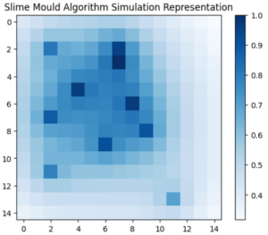
Visualizing the final positions of all agents in a 2D grid view provides insights into their exploration patterns and convergence behavior. Tracking the best solution and fitness value at each iteration allows analysis of the algorithm’s progress and convergence characteristics.
In this article, we discussed the intricate workings of the Slime Mold Algorithm (SMA), exploring its Python implementation and the magic of adaptive weights.