Optimization: Local vs. Global Optima | Baeldung on Computer Science

1. Overview

In this tutorial, we’ll talk about the concepts of local and global optima in an optimization problem. First, we’ll make an introduction to mathematical optimization. Then, we’ll define the two terms and briefly present some algorithms for computing them.

2. Prerequisites

First, let’s briefly introduce the basic terms of optimization.

A mathematical optimization problem consists of three basic components:

The objective function $f(x)$ is the value we want to optimize
The decision variables $x_1, x_2, ..., x_n$ are the inputs of the objective function we can control
The constraints $h_n(x)$ restrict the range of values the decision variables $x$ can take

So, the goal is to find the optimal values $\mathbf{x_{opt}}$ of the decision variables that satisfy the constraints and optimize (maximize or minimize) the value of $\mathbf{f(x_{opt})}$ . However, as the problem becomes more complex, finding the optimal values becomes more difficult. So, sometimes it is easier to find some values that are not optimal but are good enough for the problem. In this case, we have a local optimal.

3. Local Optima

A local optimum is an extrema (maximum or minimum) point of the objective function for a certain region of the input space. More formally, for the minimization case $x_{local}$ is a local minimum of the objective function $f$ if:

$f(x) \geq f(x_{local})$

for all values of x in range $[x_{local} - \epsilon, x_{local} + \epsilon]$ .

4. Global Optima

A global optimum is the maximum or minimum value the objective function can take in all the input space. More formally, for the minimization case $x_{global}$ is a global minimum of the objective function $f$ if:

$f(x) > f(x_{global})$

for all values of x.

In the image below, we can see an example of a local and a global maximum:

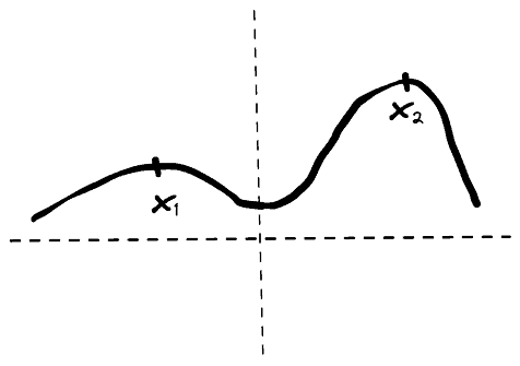
We observe that $x_2$ is the global maximum of the function since in $x_2$ , the function takes the higher value. However, if we consider only the region of negative numbers, $x_1$ is the maximum in this region. So, $x_1$ is a local maximum.

In case the objective function contains more than one global optima, the optimization problem is referred to as multimodal. In this case, there are multiple values of the decision variables $x$ that optimize the objective function.

Also, in optimization, we are interested only in cases when the objective function presents a global optimum. For example, consider the following optimization problem:

$\max{f(x)} \quad \text{where} \quad f(x) = x^2 \quad \text{and} \quad x > 0$

where we can see below the plot on the square function:

We can observe that there is no global optimum for this problem. For every $x_1 > 0$ with objective value $f(x_1) = x_1^2$ there is always a value $x_2 = x_1 + 1$ where the objective value $f(x_2)$ is greater because:

$f(x_2) = x_2^2 = (x_1 + 1)^2 = x_1^2 + 2 x_1 + 1 > x_1^2$

5. Algorithms

Generally, finding the local and global optima of a function is a very important problem, and new algorithms are proposed all the time.

In terms of local optima, some famous methods are the BFGS Algorithm, the Hill-Climbing Algorithm, and the Nelder-Mead Algorithm. In global optima computation, Simulated Annealing and Genetic Algorithms are the most successful.

However, to choose an algorithm, we should always first understand the requirements of our optimization problem since there are algorithms that aim to be fast while losing a bit of their accuracy and adversely.

6. Conclusion

In this article, we presented the terms of global and local optima. First, we briefly presented how an optimization problem is defined, and then we discussed the two terms along with some algorithms for computing them.

Full Archive

About Baeldung

Core Concepts

Operating Systems

Artificial Intelligence

Graph Theory

Latex