Find All Simple Paths Between Two Vertices in a Graph

1. Overview

In this article, we’ll discuss the problem of finding all the simple paths between two arbitrary vertices in a graph.

We’ll start with the definition of the problem. Then, we’ll go through the algorithm that solves this problem.

Finally, we’ll discuss some special cases. We’ll focus on directed graphs and then see that the algorithm is the same for undirected graphs.

2. Definition

Let’s first remember the definition of a simple path. Suppose we have a directed graph $G(V, E)$ , where $V$ is the set of vertices and $E$ is the set of edges. A simple path between two vertices $u$ and $v$ $(u \in V, v \in V)$ is a sequence of vertices $(v_1, v_2, …, v_k)$ that satisfies the following conditions:

All nodes $v_i$ where $(1 \leq i \leq k)$ belong to the set of vertices $V$
$u=v_1$ , $v=v_k$
For each two consecutive vertices $(v_i, v_{i+1})$ , where $(1 \leq i < k)$ , there is an edge $e = (v_i, v_{i+1})$ that belongs to the set of edges $E$
There is no vertex that appears more than once in the sequence; in other words, the simple path has no cycles

The problem gives us a graph and two nodes, $u$ and $v$ , and asks us to find all possible simple paths between two nodes $u$ and $v$ .

The graph can be either directed or undirected. We’ll start with directed graphs, and then move to show some special cases that are related to undirected graphs.

For example, let’s consider the graph:

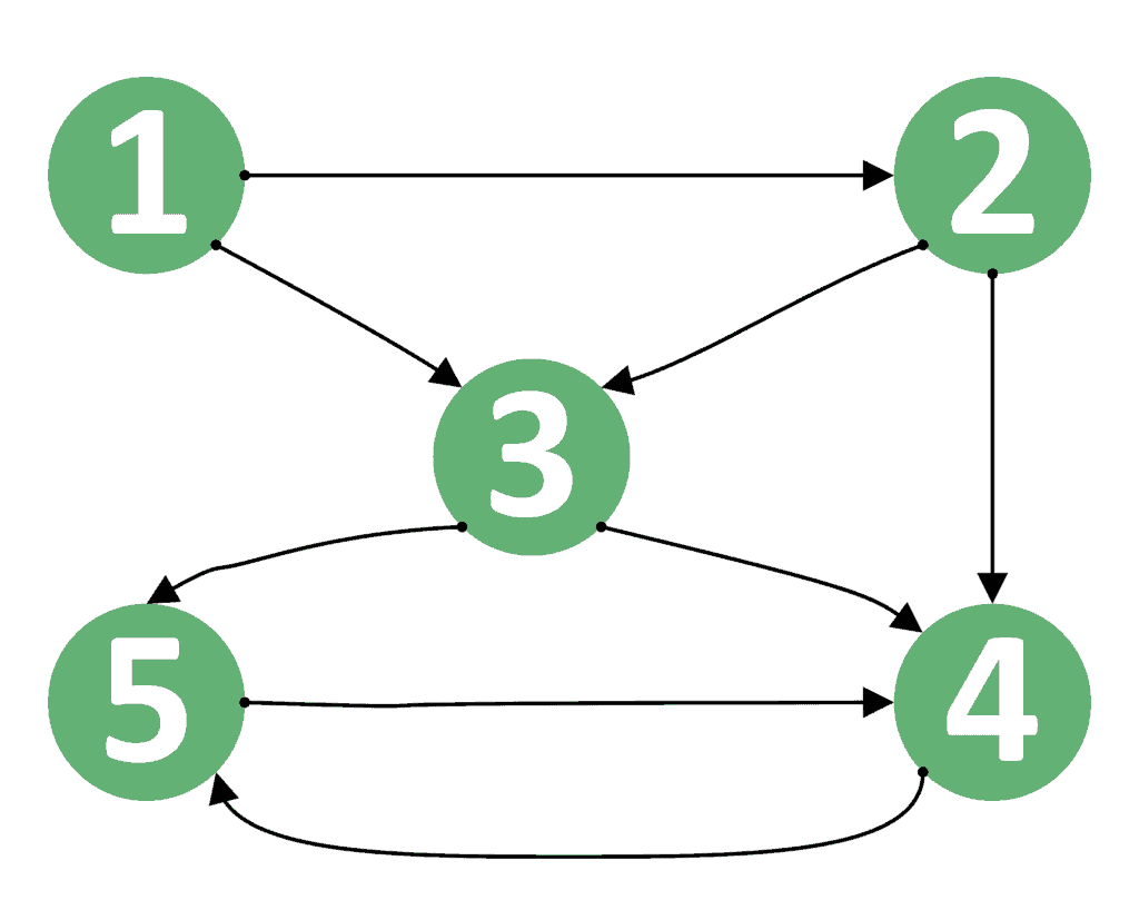
As we can see, there are 5 simple paths between vertices 1 and 4:

$(1, 2, 3, 4)$
$(1, 2, 3, 5, 4)$
$(1, 2, 4)$
$(1, 3, 4)$
$(1, 3, 5, 4)$

Note that the path $(1, 3, 4, 5, 4)$ is not simple because it contains a cycle — vertex 4 appears two times in the sequence.

3. Algorithm

3.1. Theoretical Idea

The basic idea is to generate all possible solutions using the Depth-First-Search (DFS) algorithm and Backtracking.

In the beginning, we start the DFS operation from the source vertex $u$ . Then, we try to go through all its neighbors. For each neighbor, we try to go through all its neighbors, and so on.

Hopefully, we’ll be able to reach the destination vertex $v$ . When this happens, we add the walked path to our set of valid simple paths. Then, we go back to search for other paths.

In order to avoid cycles, we must prevent any vertex from being visited more than once in the simple path. To do that, we mark every vertex as visited when we enter it for the first time in the path. Hence, when we try to visit an already visited vertex, we’ll go back immediately.

After processing some vertex, we should remove it from the current path, so we mark it as unvisited before we go back. The reason for this step is that the same node can be a part of multiple different paths. However, it can’t be a part of the same path more than once.

3.2. Implementation

Let’s take a look at the implementation of the idea we’ve just described:

algorithm findAllSimplePaths(G, u, v):
    // INPUT
    //   G = The graph stored in an adjacency list
    //   u = The starting node
    //   v = The ending node
    // OUTPUT
    //   Returns a list of all simple paths from u to v

    visited <- array of false for each node in G
    currentPath <- empty list
    simplePaths <- empty list
    DFS(u, v, visited)
    return simplePaths

function DFS(u, v, visited):
    if visited[u] = true:
        return

    visited[u] <- true
    currentPath.addToBack(u)

    if u = v:
        simplePaths.add(currentPath)
        visited[u] <- false
        currentPath.removeFromBack()
        return

    for next in G[u]:
        DFS(next, v, visited)

    currentPath.removeFromBack()
    visited[u] <- false

First of all, we initialize the $visited$ array with $false$ values, indicating that no nodes have been visited yet. Also, we initialize the $currentPath$ and $simplePaths$ lists to be empty. The $currentPath$ list will store the current path, whereas the $simplePaths$ list will store the resulting paths.

After that, we call the DFS function and then return the resulting simple paths. Let’s check the implementation of the DFS function.

First, we check whether the vertex $u$ has been visited or not. If so, then we go back because we reached a cycle. Otherwise, we add $u$ to the end of the current path using the $addBack$ function and mark node $u$ as visited.

Second, we check if vertex $u$ is equal to the destination vertex $v$ . If so, then we’ve reached a complete valid simple path. Therefore, we add this path to our result list and go back.

However, if we haven’t reached the destination node yet, then we try to continue the path recursively for each neighbor of the current vertex.

Finally, we remove the current node $u$ from the current path using a $removeBack$ function that removes the value stored at the end of the list (remember that we added the current node to the end of the list). Also, we mark the node $u$ as unvisited to allow it to be repeated in other simple paths.

3.3. Complexity

We’ll consider the worst-case scenario, where the graph is complete, meaning there’s an edge between every pair of vertices. In this case, it turns out the problem is likely to find a permutation of vertices to visit them.

For each permutation of vertices, there is a corresponding path. Hence, the complexity is $O(|V|!)$ , where $|V|$ is the number of vertices and $|V|!$ is the factorial of the number of vertices.

This complexity is enormous, of course, but this shouldn’t be surprising because we’re using a backtracking approach.

4. Undirected Graphs

The previous algorithm works perfectly fine for both directed and undirected graphs. The reason is that any undirected graph can be transformed to its equivalent directed graph by replacing each undirected edge $(u - v)$ with two directed edges $(u -> v)$ and $(v -> u)$ .

However, in undirected graphs, there’s a special case where the graph forms a tree. We’ll discuss this case separately.

5. Trees

Remember that a tree is an undirected, connected graph with no cycles.

In this case, there is exactly one simple path between any pair of nodes inside the tree. Specifically, this path goes through the lowest common ancestor (LCA) of the two nodes. In other words, the path starts from node $u$ , keeps going up to the LCA between $u$ and $v$ , and then goes to $v$ .

For example, let’s take the tree shown below:

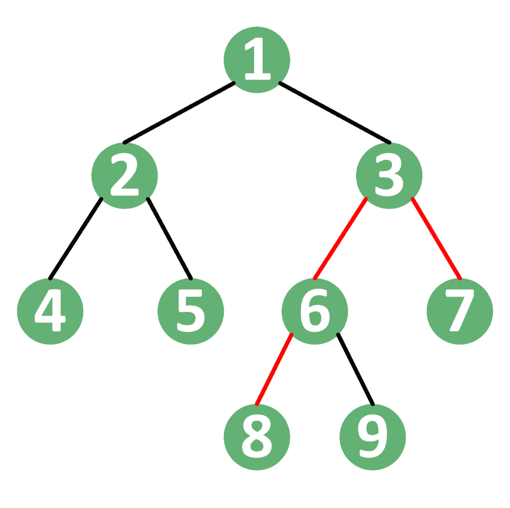
In this tree, the simple path between nodes 7 and 8 goes through their LCA, which is node 3. Similarly, the path between nodes 4 and 9 goes through their LCA, which is node 1.

6. Disconnected Undirected Graphs Without Cycles

In the general case, undirected graphs that don’t have cycles aren’t always connected. If the graph is disconnected, it’s called a forest. A forest is a set of components, where each component forms a tree itself.

When dealing with forests, we have two potential scenarios. For one, both nodes may be in the same component, in which case there’s a single simple path. The reason is that both nodes are inside the same tree.

On the other hand, if each node is in a different tree, then there’s no simple path between them. This is because each node is in a different disconnected component.

For example, take a look at the forest below:

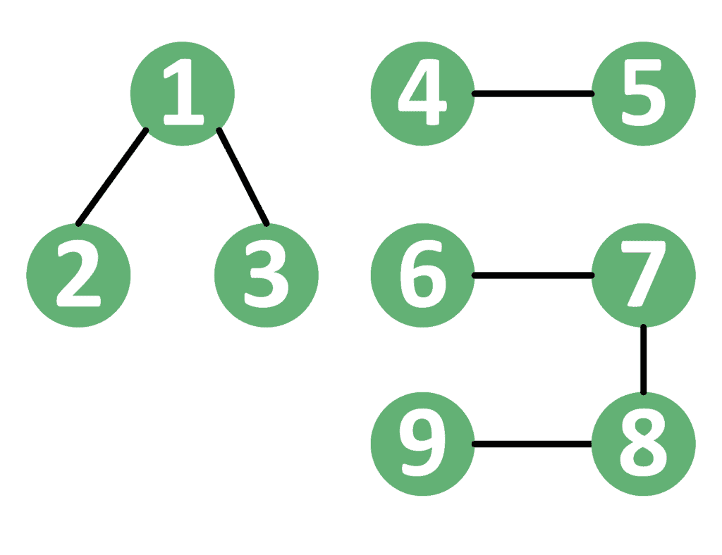
In this graph, there’s a simple path between nodes 2 and 3 because both are in the same tree containing nodes { $1, 2, 3$ }. However, there isn’t any simple path between nodes 5 and 8 because they reside in different trees.

7. Conclusion

In this tutorial, we’ve discussed the problem of finding all simple paths between two nodes in a graph.

In the beginning, we started with an example and explained the solution to it. After that, we presented the algorithm along with its theoretical idea and implementation.

Finally, we explained a few special cases that are related to undirected graphs.

Full Archive

About Baeldung

Core Concepts

Operating Systems

Artificial Intelligence

Graph Theory

Latex