Lowest Common Ancestor of Two Nodes in a Tree | Baeldung on Computer Science

1. Overview

In this article, we’ll discuss the Lowest Common Ancestors problem. We’ll start with the basic definition, then go through some of the methods used to find the lowest common ancestor of two nodes in a rooted tree.

2. Definition

The Lowest Common Ancestor (LCA) of two nodes $u$ and $v$ in a rooted tree is the lowest (deepest) node that is an ancestor of both $u$ and $v$ .

Remember that an ancestor of a node $x$ in a rooted tree is any node that lies on the path from the root to $x$ (including $x$ ).

For example, let’s look at the following tree, which is rooted at node 1:

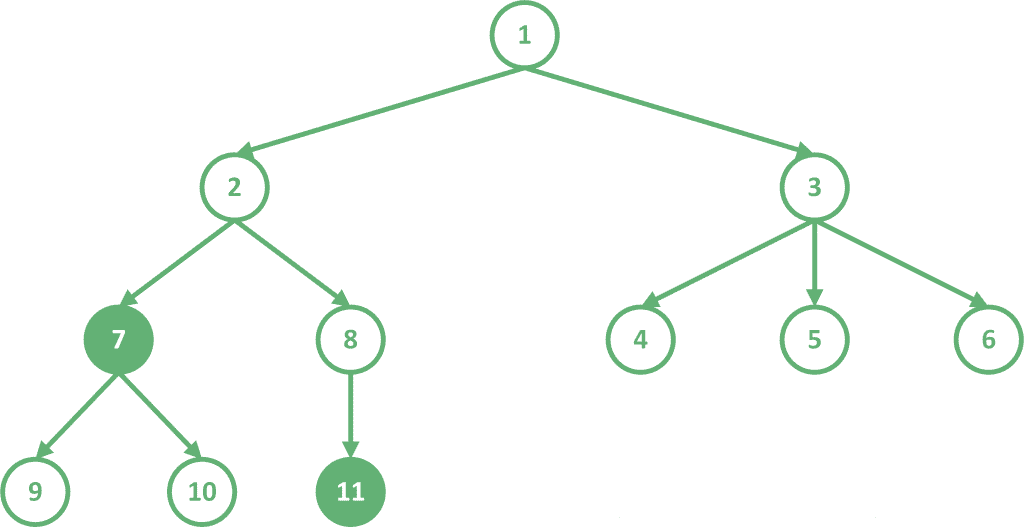
Let’s find the LCA of the two highlighted nodes 7 and 11. The common ancestors of these two nodes are nodes 1 and 2. Since node 2 is deeper than node 1, $LCA(7,11)=2$ .

3. Naive Approach

3.1. Theoretical Idea

The idea of this approach is to have two pointers, one on each node. We need to move these pointers towards the root in a way that allows them to meet at the LCA.

The first thing we can notice is that these pointers should be in the same depth. In addition to that, the deeper pointer can never be the LCA. Therefore, our first step should be to keep moving the deeper pointer to its parent until the two pointers are on the same depth.

Now, we have two pointers that are on the same depth. We can keep moving both pointers towards the root one step at a time until they meet at one node. Since this node is the deepest node that our pointers can meet at, therefore, it’s the deepest common ancestor of our starting nodes, which is the LCA.

3.2. Preprocessing

In order to implement this solution, we will need to calculate the depth and the parent of each node. This can be done with a simple DFS traversal starting from the root.

Firstly, we set the current node as visited. Secondly, we set the parent and depth of the child node before calling the function recursively for it.

The complexity of the preprocessing step in this approach is $O(n)$ , where $n$ is the number of nodes. The complexity is considered efficient because we only need to apply it once.

3.3. Finding the LCA

After calling the previous function starting from the root, we will have the depth and parent of each node. We can now apply the approach that we discussed earlier.

First of all, we keep moving the deeper node to its parent until both nodes have the same depth. After that, we move both nodes to their parents until they meet.

Although the approach is considered fairly simple, however, finding the LCA of a pair of nodes also has a complexity of $O(h)$ , where $h$ is the height of the tree. This complexity can go as far as becoming $O(n)$ in case of an almost linear tree (consider two long chains connected at the root).

4. Sparse Table Background

In order to enhance our approach discussed in section 3, we need to present some background on the sparse table data structure. The sparse table has to be built first. Then, it can then answer minimum range queries in a low complexity.

We’ll discuss the main idea of the sparse table. Later, we’ll update it to fit our needs.

4.1. Building the Sparse Table

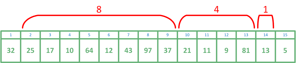
A sparse table is a data structure capable of answering range queries on static arrays in $O(log(n))$ with $O(n \cdot log(n))$ preprocessing. The intuition behind this data structure is that any range can be represented as a concatenation of at most $log(n)$ ranges whose lengths are powers of two. This is equivalent to representing the length of the range in binary. For example, a range of length $13$ can be represented as the concatenation of three ranges with lengths 8, 4, and 1.

Let’s discuss a sparse table used to answer minimum range queries in an array $Arr$ . The sparse table will consist of a $2D$ array $ST$ of size $N \cdot log(n)$ . $ST[i][j]$ will store the minimum value in the range that starts at the $i^{th}$ element of the array and has a length of $2^j$ .

Let’s fill this array in increasing order of $j$ :

$ST[i][0]$ is simply equal to $Arr[i]$ .
Let’s calculate $ST[i][j]$ for $j>1$ : We know that this value is the minimum value in the range with length $2^j$ starting at index $i$ . We can break this range into two equal parts, each of length $2^{j-1}$ , one starting at $i$ , and the other one starting at $i+2^{j-1}$ . This means that $ST[i][j]$ is equal to the minimum value between $ST[i][j-1]$ and $ST[i+2^{j-1}][j-1]$ .

Take a look at the implementation of the algorithm.

The complexity of building the sparse table is $O(n \cdot log(n))$ , where $n$ is the number of elements.

4.2. Querying the Sparse Table

Now that we have the sparse table built, let’s look at how we can answer range minimum queries using it. One way to convert a number $X$ into binary is to go through the powers of two in decreasing order. If the current power is less than or equal to $X$ , activate the corresponding bit and subtract it from $X$ . We’ll be doing something similar. Let’s say we want to find the minimum value in the range $[l,r]$ .

First, our current location is at $l$ . We want to find the largest $2^j$ such that $l + 2^j - 1 \leq r$ (longest range whose length is a power of 2 and contained in $[l,r]$ ). After finding this value, we can get the minimum value in this range in $O(1)$ since it is already stored in $ST[l][j]$ .

Next, we have to find the minimum value in the range $[l+2^j, r]$ in the same way. We keep doing this until we end up with an empty interval. The values of $j$ will be strictly decreasing, so one loop through values of $j$ in decreasing order will be enough to calculate the answer.

Let’s have a look at the described algorithm.

The complexity of querying the sparse table is $O(log(n))$ , where $n$ is the number of elements.

Now that we have some background on how sparse tables work, we can take a look at a more efficient algorithm to find the LCA.

5. Binary Lifting Approach

5.1. Theoretical Idea

Let’s build a structure similar to a sparse table, but instead of storing the minimum/maximum value in a range whose length is a power of two, it will store the ${2^{j}}^{th}$ ancestor of each node for every $0 \leq j \leq log(n)$ .

In other words, if we had a pointer to some node $v$ , and moved this pointer to its parent $2^j$ times, we will end up at node $ST[x][j]$ . Let’s call this a $2^j$ jump from $x$ .

5.2. Preprocessing

Before we start building this structure, we need an array $Par$ that stores the immediate parent of each node.

Building the structure is similar to building a normal sparse table:

$ST[i][0] = Par[i]$
To find the value of $ST[i][j]$ for $j>1$ , we need to do a $2^j$ jump from $i$ . However, we already know that if we do a $2^{j-1}$ jump from $i$ , we will end up at node $x = ST[i][j-1]$ . We also know that if we do a $2^{j-1}$ jump from $x$ , we will end up at node $ST[x][j-1]$ . Since two consecutive $2^{j-1}$ jumps are equivalent to a $2^j$ jump, this means that $ST[i][j] = ST[x][j-1] = ST[ST[i][j-1]][j-1]$ .

5.3. Algorithm

Now, let’s see how we can use the sparse table structure to optimize the naive approach. The naive approach consisted of two main steps.

The first step was to move the deeper pointer to its parent until both pointers are on the same depth.

Let’s assume that the deeper pointer is at node $u$ , and the other one is at node $v$ . We need to move the pointer $u$ a known amount of steps which is equal to $Need = Depth[u] - Depth[v]$ . If we convert $Need$ into binary, and do $2^i$ jumps for every $i$ such that the $i^{th}$ bit is activated, we would end up with a $Need$ jump. This jump would put this pointer on the same depth as the other pointer.

Since each jump is $O(1)$ and we need to check $log(n)$ types of jumps, this whole step has a complexity of $O(log(n))$ .

The second step was to move both pointers simultaneously until they meet at some node.

The main idea here is to try a huge jump at first. If doing a huge jump on both pointers leads them to the same node, then we have arrived at a common ancestor. However, we may have jumped too far. There could be some deeper common ancestor. So we can’t do this jump, let’s try something smaller.

If the current jump leads them to different nodes, then we should do this jump and update the pointers. This basically means that we made the largest possible jump that doesn’t reach any common ancestor yet. Therefore, the parent of both pointers will be the deepest common ancestor, which is the LCA. During this step, we also consider $log(n)$ different jumps, so the complexity is also $O(log(n))$ .

The complexity of this algorithm is $O(log(n))$ , where $n$ is the number of nodes.

5.4. Binary Lifting Algorithm Steps

To recap, finding the LCA with this approach consists of two main parts:

Preprocessing: This part will only be applied once on the tree, and has two steps:
- Find the depth and the parent of each node (Algorithm 1).
- Build the sparse table structure (Algorithm 5).
  The complexity of this part is $O(n \cdot log(n))$ due to the complexity of building the sparse table.
Answer LCA Query: This part will be applied for each pair of nodes that we want to find the LCA for (Algorithm 6).
The complexity of this part is $O(log(n))$ since we are only doing $O(log(n))$ jumps.

6. Comparison

Let’s have a final comparison between the two approaches in this tutorial.

The main bonus when using the binary lifting approach is that we can handle a large number of queries. First, we have to apply the preprocessing once, and then we can have a large number of queries, where each query is answered in $O(log(n))$ . Therefore, each query will be answered in a better complexity than when using the naive approach.

7. Conclusion

In this tutorial, we’ve discussed the Least Common Ancestors problem for tree data structures.

First, we took a look at the definition, then discussed two methods of finding the LCA. Finally, we did a simple comparison between the two methods.

Full Archive

About Baeldung

Core Concepts

Operating Systems

Artificial Intelligence

Graph Theory

Latex