

Learn through the super-clean Baeldung Pro experience:
>> Membership and Baeldung Pro.
No ads, dark-mode and 6 months free of IntelliJ Idea Ultimate to start with.
Last updated: March 18, 2024
Learn through the super-clean Baeldung Pro experience:
>> Membership and Baeldung Pro.
No ads, dark-mode and 6 months free of IntelliJ Idea Ultimate to start with.
In this tutorial, we’ll discuss finding the shortest path in a graph visiting all nodes.
First, we’ll define the problem and provide an example that explains it. Then, we’ll discuss two different approaches to solve this problem.
Suppose we have a graph,  , that contains
  nodes numbered from
  to
to  . In addition, we have
  edges that connect these nodes. Each of these edges has a weight associated with it, representing the cost to use this edge.
Our task is to find the shortest path that goes through all nodes in the given graph.
Recall that the shortest path between two nodes  and
and  is the path that has the minimum cost among all possible paths between and .
In this task, we look for all the paths that cover all possible starting and ending nodes. Besides, we can visit the same node more than once. Let’s look at an example for better understanding.
Suppose we have the following graph:
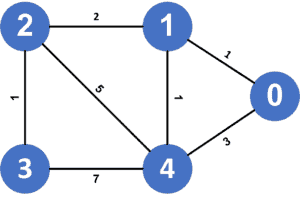
As we can see, there’re many paths that go through all nodes in the given graph, but the shortest path among them  , and it has a cost equal to
  ; therefore, the shortest path in the given graph visiting all nodes has a cost equal to
  .
.
The main idea here is to generate all the possible paths and get the one that has the minimum cost.
Firstly, we’ll generate all the possible permutations of nodes. Each permutation will represent the order of visiting nodes in the graph. A path’s cost will be equal to the sum of all shortest paths between every two consecutive nodes.
Secondly, we’ll calculate the shortest path between every two consecutive nodes using the Floyd-Warshall algorithm. Recall that the Floyd-Warshall algorithm calculates the shortest path between all pairs of nodes inside a graph.
Finally, the shortest path visiting all nodes in a graph will have the minimum cost among all possible paths.
Let’s take a look at the implementation:
algorithm BruteForceApproach(V, G):
    // INPUT
    //     V = the number of nodes in the graph
    //     G = the graph stored as an adjacency list
    // OUTPUT
    //     Returns the shortest path visiting all nodes in G

    answer <- infinity
    distance <- Calculate_Floyd_Warshall(G) // a matrix
    permutations <- Calculate_Permutations()

    for permutation in permutations:
        cost <- 0
        previous <- permutation[0]
        for node in permutation:
            cost <- cost + distance[previous, node]
            previous <- node
        if cost < answer:
            answer <- cost

    return answer
Initially, we declare an array called  , which stores the shortest path between every pair of nodes in the given graph using the Floyd-Warshall algorithm.
Next, we generate all the possible permutation which represent all the possible paths we could follow. Then for each permutation, we’ll calculate the cost of it by adding the length of the shortest path between every two consecutive nodes; after calculating the cost of the current permutation, we’ll check if the  is less than the
  value, then we’ll update the .
Finally, we return , which stores the cost of the shortest path visiting all nodes in the given graph.
The time complexity here is  . Let’s examine the reason behind this complexity.
First, the Floyd-Warshall algorithm has complexity  . Next, the number of all different permutations of nodes is equal to the factorial of , and for each permutation, we calculate its cost by passing through it, so it’s
  .
.
Therefore, the total complexity will be  .
.
In this approach, we’ll use a modified version of the Dijkstra algorithm. For each state, we need to keep track of all the visited nodes besides the current one. So, to get all the visited nodes in each state, we’ll represent them as bitmask where each bit that’s turned on means that we’ve visited this node before.
In the end, our answer we’ll be the minimum value among all nodes’ values that have a bitmask full of ones (visited all nodes).
Let’s take a look at the implementation:
algorithm DijkstraApproach(V, G):
    // INPUT
    //     V = the number of nodes in the graph
    //     G = the graph stored as an adjacency list
    // OUTPUT
    //     Returns the shortest path visiting all nodes

    cost <- a matrix whose all entries are infinity
    priority_queue <- make an empty priority queue
    for node from 0 to V-1:
        priority_queue.add(node, 2^node)
        cost[node, 2^node] <- 0

    while priority_queue is not empty:
        current <- priority_queue.front().node
        mask <- priority_queue.front().bitmask
        priority_queue.pop()
        for child in G[current]:
            add <- weight(current, child)
            if cost[child, mask or 2^child] > cost[current, mask] + add:
                priority_queue.add(child, mask or 2^child)
                cost[child][mask or 2^child] <- cost[current][mask] + add

    answer <- infinity
    for node from 0 to V-1:
        answer <- min(answer, cost[node, 2^V - 1])

    return answer
Initially, we declare an array called , which stores the shortest path to some node visiting a subset of nodes. We also declare a priority queue that stores a node and a bitmask. The bitmask represents all visited nodes to get to this node. This priority queue will sort states in acceding order according to the cost of the state.
Next, we try to start the shortest path from each node by adding each node to the priority queue and turning their bit on. Then, we run the Dijkstra algorithm.
We iterate over the children nodes of the  node. For each
  , we check if the value of it visiting a specific subset of nodes greater than the current plus the weight of the edge that connects the node with the . In this case, we need to update the value of the node. Also, we add the and the current
  bitwise-or
  to the priority queue. This mask means that we turn the bit of the node on.
Finally, our answer will be the minimum value among all the nodes cost visiting all nodes.
The time complexity here is  , where is the number of nodes and
  is the number of all possible subset of nodes, and
  for adding each state to the priority queue.
In this article, we presented the problem of finding the shortest path visiting all nodes. We explained the main ideas behind two different approaches to solving this problem and walked through their implementation.