Understanding the Randomized Quicksort | Baeldung on Computer Science

1. Overview

In this tutorial, we’ll discuss the randomized quicksort. In the beginning, we’ll give a quick reminder of the quicksort algorithm, explain how it works, and show its time complexity limitations. Next, we’ll present two adjustments that can be made to apply the randomized quicksort algorithm.

2. Quicksort

Let’s quickly remind how quicksort works and how it chooses a pivot element. Then, we’ll discuss the cases when the best and worst time complexity occurs and what is the overall time complexity of the algorithm.

2.1. Choosing a Pivot

The quicksort algorithm performs multiple steps. Each step chooses a pivot element and places it in its correct location. Placing the pivot element in its correct location means comparing it to all the other elements, counting the number of elements that are smaller or larger than the pivot, and then placing it between all the elements that are smaller to its left and the ones that are larger to its right.

Take a look at the following example:

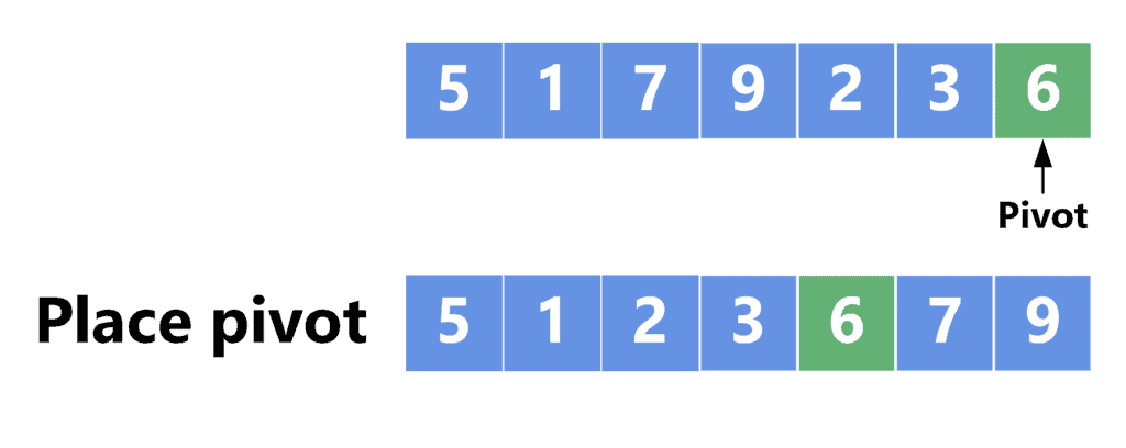
In this example, we chose the last element as the pivot. After that, we put all the elements that are smaller than the pivot at the beginning of the array, place the pivot in its correct location, and put all the larger elements at the end of the array.

Note that we can only guarantee to have the pivot in its correct location because we don’t sort the other elements. Instead, we move them to the left or right of the pivot. Finally, we perform two recursive calls. The first call sorts the elements before the pivot, while the other sorts the ones after.

The time complexity of the quicksort algorithm depends on the chosen pivot in each step. Let’s show this more closely with some examples.

2.2. Best-Case Scenario

The best-case scenario occurs when the pivot element divides the array in half. Moreover, when the recursive calls are made, it’s best if the pivot element divides the range of each recursive call in half. Take a look at the following example:

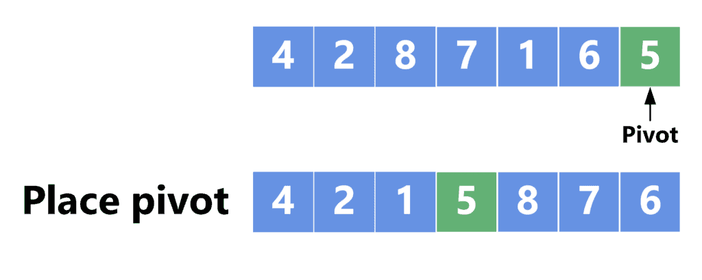
In this example, we chose the pivot element as the last one. In this case, after placing the pivot element in its correct location, the array was divided in half. Therefore, when we make the recursive calls, we’ll make them into ranges $[0, 2]$ and $[4, 6]$ .

The reason that this is the best-case scenario is that if we keep dividing the array in half, we’ll end up with the minimum number of recursion levels, which is $\mathbf{O(log(n))}$ levels, where $\mathbf{n}$ is the size of the array. Since in each level, we perform $O(n)$ comparisons to put the pivot in its correct location, then the overall complexity in the best-case scenario is $O(n \cdot log(n))$ .

2.3. Worst-Case Scenario

On the other hand, the worst-case scenario occurs when the array is not divided by half, and the recursive calls are made to an array of size zero and an array of size $n - 1$ , where $n$ is the number of elements in the original array.

This occurs when the pivot is either the smallest or the largest element in the array. Take a look at the following example:

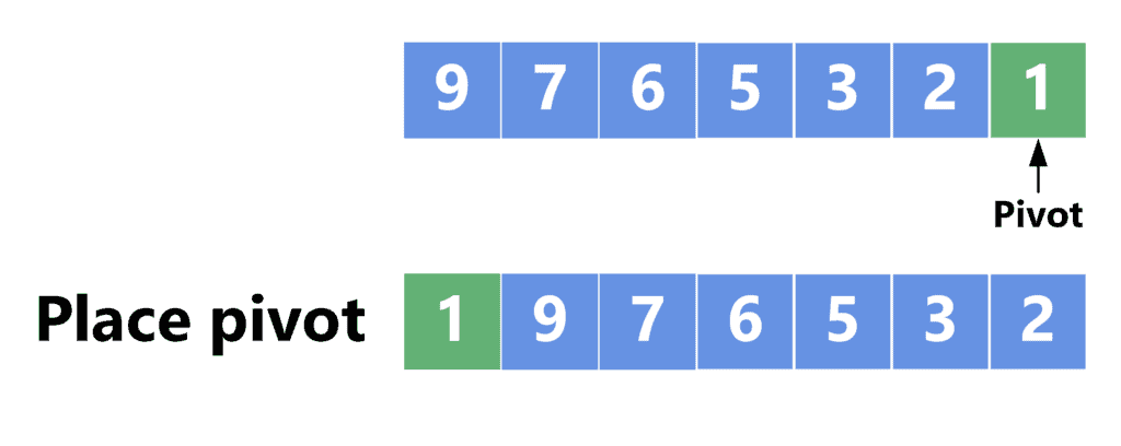
Choosing the pivot as the last element, in this case, results in it being the smallest one. Thus, it’s placed at the first position inside the array. Since all other elements are larger than the pivot element, they are placed in the remaining part of the array. Now, we make only one recursive call for the range $[1, n - 1]$ .

Since each recursive call reduces the size of the array by one, we’ll have $O(n)$ recursive levels after all. Since each level contains $O(n)$ comparisons to put the pivot in its correct location, the overall time complexity will be $\mathbf{O(n^2)}$ .

2.4. Reducing the Worst-Case Scenario

As we discussed, the overall time complexity for the quicksort algorithm varies between the best-case and the worst-case scenarios. More formally, the complexity can be given using the formula:

$\mathbf{O(n \cdot log(n)) \leq complexity \leq O(n^2)}$

This difference depends on the chosen pivot elements. Since the worst-case scenario occurs when the pivot is the smallest or largest element, we try to reduce this case from occurring by using a random approach for choosing the pivot element. We’ll present two approaches to achieve that.

3. Random Shuffle Approach

The random shuffle approach uses the same location for the pivot element throughout all the steps of the algorithm. For example, it’ll stick to picking the last element of each range as the pivot element in all the recursive calls.

However, This approach performs a random shuffle on the array before choosing the pivot element. Thus, it reduces the probability of picking a pivot element that can cause the worst-case scenario. Consider the following example:

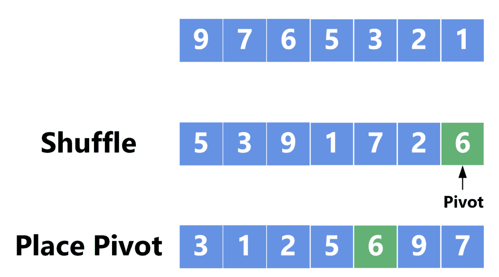
Performing the quicksort on an array already sorted in ascending or descending order will result in the worst-case scenario. In the example above, choosing the last element $array[6] = 1$ as the pivot from the first array immediately will place it at the beginning of the array and will result in a recursive call for the range $[1, 6]$ .

However, performing a random shuffle on the array before choosing the pivot element will cause a higher probability of choosing a different element as the pivot. Thus, we’ll end up with a more balanced distribution of the elements on the sides of the pivot.

4. Random Pivot Selection

Another way to reduce the probability of the worst-case scenario is to choose the pivot element randomly at each step. More formally, the pivot element can be chosen using the following equation:

$\mathbf{pivot = L + (random() \mod (R - L + 1))}$

Where $L$ is the index of the first element in the range, and $R$ is the index of the last element in the range. Therefore, we generate a random number using the function $random()$ and take that number modulo the length of the range, which is $R - L + 1$ . This resulting index will be zero-based. Thus, we shift it by $L$ to the corresponding range.

Let’s take a look at the following example:

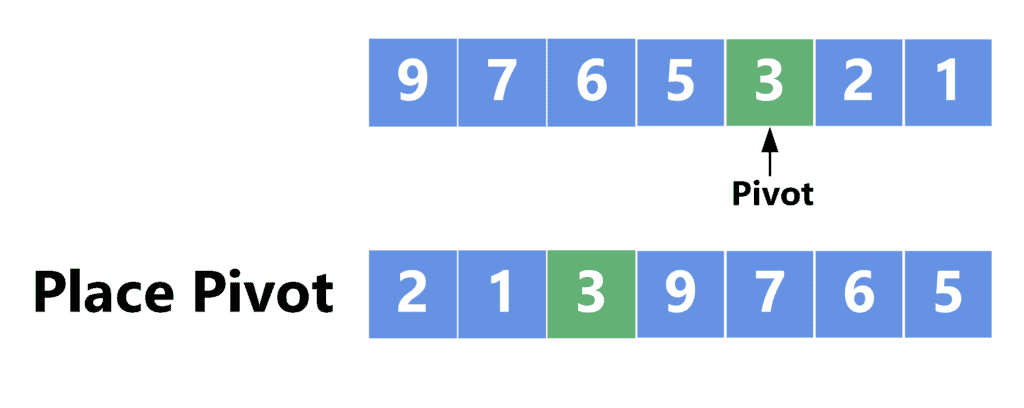
Choosing the pivot as the last element would result in the worst-case scenario. However, choosing it randomly can produce $array[4] = 3$ , which divides the array in a better way.

5. Comparison

Both random shuffle and pivot selection approaches can be used to choose the pivot element. However, the random shuffle adds more complexity to the process due to the following facts:

Shuffling the array requires an auxiliary array to put the shuffled elements to. Thus, it results in added memory complexity
In the best case, shuffling an array takes $O(n)$ time complexity. After choosing the pivot, we still make $O(n)$ comparisons, which means that shuffling doesn’t add time complexity when considered in the big-O notation. However, it still adds operation, which results in a slower runtime for the algorithm

On the other hand, the random pivot selection approach doesn’t add any additional memory or time complexity. The reason is that the pivot index is calculated in $O(1)$ , without performing any comparisons or operations.

Therefore, we prefer the random pivot selection over the random shuffle approach.

6. Conclusion

In this tutorial, we discussed the randomized quicksort algorithm. We started by reminding us how the quicksort algorithm works and presenting the best and worst-case scenarios for the algorithm’s time complexity.

After that, we presented two approaches to reduce the probability of the worst-case scenario and summarized with a comparison between both approaches.

Full Archive

About Baeldung

Core Concepts

Operating Systems

Artificial Intelligence

Graph Theory

Latex