Fastest Algorithm to Find Prime Numbers | Baeldung on Computer Science

1. Overview

Prime numbers have always been an interesting topic to dive into. However, no one has been able to find a clean and finite formula to generate them. Therefore, mathematicians have relied on algorithms and computational power to do that. Some of these algorithms can be time-consuming while others can be faster.

In this tutorial, we’ll go over some of the well-known algorithms to find prime numbers. We’ll start with the most ancient one and end with the most recent one.

Most algorithms for finding prime numbers use a method called prime sieves. Generating prime numbers is different from determining if a given number is a prime or not. For that, we can use a primality test such as Fermat primality test or Miller-Rabin method. Here, we only focus on algorithms that find or enumerate prime numbers.

2. Sieve of Eratosthenes

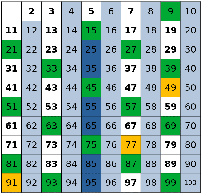
Sieve of Eratosthenes is one of the oldest and easiest methods for finding prime numbers up to a given number. It is based on marking as composite all the multiples of a prime. To do so, it starts with $2$ as the first prime number and marks all of its multiples ( $\texttt{4, 6, 8, ...}$ ). Then, it marks the next unmarked number ( $\texttt{3}$ ) as prime and crosses out all its multiples ( $\texttt{6, 9, 12, ...}$ ). It does the same for all the other numbers up to $n$ :

However, as we can see, some numbers get crossed several times. In order to avoid it, for each prime $p$ , we can start from $p^2$ to mark off its multiples. The reason is that once we get to a prime $p$ in the process, all its multiples smaller than $p^2$ have already been crossed out. For example, let’s imagine that we get to $7$ . Then, we can see that $\texttt{14, 21, 28, 35,}$ and $\texttt{42}$ have already been marked off by $\texttt{2, 3, 2, 5,}$ and $\texttt{3}$ . As a result, we can begin with $\texttt{49}$ .

We can write the algorithm in the form of pseudocode as follows:

In order to calculate the complexity of this algorithm, we should consider the outer $\texttt{for}$ loop and the inner $\texttt{while}$ loop. It’s easy to see that the former’s complexity is $O(\sqrt{n})$ . However, the latter is a little tricky. Since we enter the $\texttt{while}$ loop when $i$ is prime, we’ll repeat the inner operation $\frac{\sqrt{n}}{p}$ number of times, with $p$ being the current prime number. As a result, we’ll have:

$\sqrt{n} \sum_{p<\sqrt{n}} \frac{\sqrt{n}}{p} = n \sum_{p<\sqrt{n}} \frac{1}{p}$

In their book (theory of numbers), Hardy and Wright show that $\sum_{p<n} \frac{1}{p} = \texttt{log\,log\,n} + O(1)$ . Therefore, the time complexity of the sieve of Eratosthenes will be $O(\texttt{n\,log\,log\,n})$ .

3. Sieve of Sundaram

This method follows the same operation of crossing out the composite numbers as the sieve of Eratosthenes. However, it does that with a different formula. Given $i$ and $j$ less than $n$ , first we cross out all the numbers of the form $i + j + 2ij$ less than $n$ . After that, we double the remaining numbers and add $1$ . This will give us all the prime numbers less than $2n + 1$ . However, it won’t produce the only even prime number ( $2$ ).

Here’s the pseudocode for this algorithm:

We should keep in mind that with $n$ as input, the output is the primes up to $2n + 1$ . So, we divide the input by half, in the beginning, to get the primes up to $n$ .

We can calculate the complexity of this algorithm by considering the outer $\texttt{for}$ loop, which runs for $\sqrt{n}$ times, and the inner $\texttt{while}$ loop, which runs for less than $\frac{\sqrt{n}}{i}$ times. Therefore, we’ll have:

$\sqrt{n} \sum_{i<\sqrt{n}} \frac{\sqrt{n}}{i} = n \sum_{i<\sqrt{n}} \frac{1}{i}$

This looks like a lot similar to the complexity we had for the sieve of Eratosthenes. However, there’s a difference in the values $i$ can take compared to the values of $p$ in the sieve of Eratosthenes. While $p$ could take only the prime numbers, $i$ can take all the numbers between $1$ and $\sqrt{n}$ . As a result, we’ll have a larger sum. Using the direct comparison test for this harmonic series, we can conclude that:

$\sum_{i=1}}^{i=\sqrt{n}} \frac{1}{i} \geq 1 + \frac{\texttt{log\,n}}{4}$

As a result, the time complexity for this algorithm will be $O(\texttt{n\,log\,n)}$ .

4. Sieve of Atkin

Sieve of Atkin speeds up (asymptotically) the process of generating prime numbers. However, it is more complicated than the others.

First, the algorithm creates a sieve of prime numbers smaller than 60 except for $\texttt{2, 3, 5}$ . Then, it divides the sieve into $3$ separate subsets. After that, using each subset, it marks off the numbers that are solutions to some particular quadratic equation and that have the same modulo-sixty remainder as that particular subset. In the end, it eliminates the multiples of square numbers and returns $\texttt{2, 3, 5}$ along with the remaining ones. The result is the set of prime numbers smaller than $n$ .

We can express the process of the sieve of Atkin using pseudocode:

It is easy to see that the first three $\texttt{for}$ loops in the sieve of Atkin require $O(n)$ operations. To conclude that the last loop also runs in $O(n)$ time, we should pay attention to the condition that will end the loop. Since when $m^2$ and $c$ , which is a multiple of a square number, are greater than $n$ , we get out of the loops, they both run in $O(\sqrt{n})$ time. As a result, the asymptotic running time for this algorithm is $O(\texttt{n})$ .

Comparing this running time with the previous ones shows that the sieve of Atkin is the fastest algorithm for generating prime numbers. However, as we mentioned, it requires a more complicated implementation. In addition, due to its complexity, this might not even be the fastest algorithm when our input number is small but if we consider the asymptotic running time, it is faster than others.

5. Conclusion

In this article, we reviewed some of the fast algorithms that we can use to generate prime numbers up to a given number.

Full Archive

About Baeldung

Core Concepts

Operating Systems

Artificial Intelligence

Graph Theory

Latex

1. Overview

2. Sieve of Eratosthenes

3. Sieve of Sundaram

4. Sieve of Atkin

5. Conclusion