

Learn through the super-clean Baeldung Pro experience:
>> Membership and Baeldung Pro.
No ads, dark-mode and 6 months free of IntelliJ Idea Ultimate to start with.
Last updated: March 18, 2024
Learn through the super-clean Baeldung Pro experience:
>> Membership and Baeldung Pro.
No ads, dark-mode and 6 months free of IntelliJ Idea Ultimate to start with.
Networking is the backbone of all modern internet applications. As such, user experience depends heavily on the network’s performance and reliability.
However, networks are by no means perfectly operational constructs. Their flaws include but are not limited to packet delays, collisions, and losses. Therefore, we need to be able to factor these phenomena into our calculations.
In this tutorial, we’ll be discussing packet transmission time and how we can approximately calculate it.
There are several factors that delay the transmission of a packet. In this article, we’re going to be discussing the 4 main ones, namely processing delay, queuing delay, transmission delay, and propagation delay.
Networks can be accurately modeled as graphs, where nodes represent devices such as computers, routers, switches, etc., and edges represent established links between these devices.
For the sake of simplicity, let us first consider an example network as shown in the image below and assume that a packet has just reached node A before heading to node B:
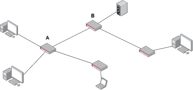
All the potential delays associated with the transmission from A to B can, of course, be trivially generalized to more complex paths.
Upon reaching node A, the packet’s header has to be processed. First, bit-level errors that might have occurred during transmission to node A must be located and corrected.
Next, the packet’s header must also be examined to determine the correct link that the packet must be forwarded to in order to reach node B. This is an important step, as the current node might be part of multiple links, connecting it to different devices.
After the appropriate link is found, the packet is pushed into the queue, waiting to be transmitted onto the wire.
Every router contains an internal buffer in which packets are placed after being processed. Since routers can only transmit one packet at a time, if a new packet arrives while an old one is still being transmitted, the packet will have to be placed inside this buffer while it waits:
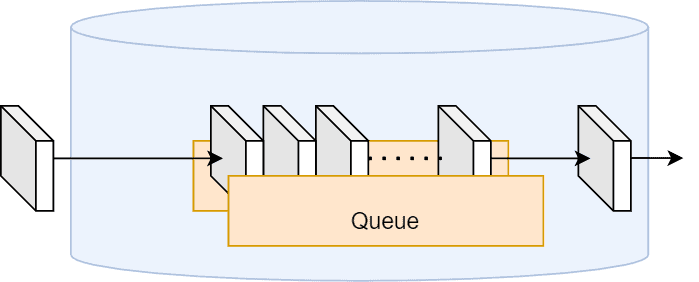
This buffer is called the queue. Routers follow a “first come, first served” policy, so packets that have arrived first will also be transmitted first.
Queuing delays can span from just a few microseconds all the way to milliseconds depending on the network traffic. During rush hour, queuing delays can significantly impact the total delay of packets, especially when retransmission due to packet loss is taken into account.
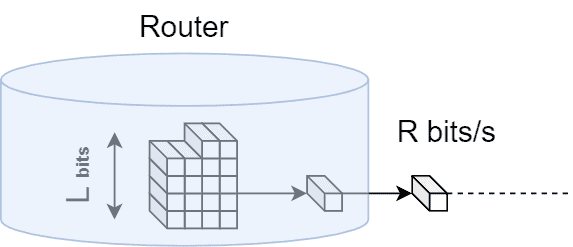
We have used the word “transmission” quite extensively in this article to symbolize the entire process of a packet going from node A to node B. However, transmission delay refers to the time required for an entire packet to be sent onto the wire, bit by bit.
Naturally, this type of delay depends on the transmission rate of the link. For example, sending a packet comprised of L bits through a link with transmission rate R would amount to a transmission delay of L/R:
The final delay component we’ll be discussing is the propagation delay. As the name implies, it is the time required for a bit to travel from node A to B after being pushed onto the physical medium.
It depends on two factors, the distance d between the nodes, as well as the propagation speed associated with that particular medium. The propagation speed is generally very high, usually ranging between  , where
  is the speed of light.
The total node delay for a packet to be transmitted is the sum of all the aforementioned delay terms:  . In practice however, not all terms of this expression are equally important, rather it heavily depends on the situation.
For example, the propagation delay is negligible during a LAN party with friends but is quite significant for nodes connected via a satellite link.
Transmission delay is rarely an issue nowadays. This is because gigabit ethernet and optical fiber links guarantee very high transmission rates. This is certainly not the case for old modems, however, where low throughput, analog telephony links are used.
Routers contain dedicated hardware with a high enough processing power, so processing delays are usually insignificant in practice.
Arguably the most influential and important factor is the queuing delay. Consecutive packets in the queue will have a different delay, depending on their order. The first packet will be transmitted immediately, whereas the 10th packet will have to wait for the 9 packets in front of it to be transmitted. That’s why we usually talk in terms of expected value when we discuss queuing delays.
Let us review what we learned by taking a look at a numerical problem.
Packets of length  bits arrive in waves at router A and are placed in the queue while awaiting transmission to node B. The transmission rate of the link is
  . Each wave contains
  packets, and a single wave arrives every
  . Processing delays are negligible and are not taken into account.
 and the propagation speed is
For a packet inside the queue to be transmitted, all packets that are in front of it have to be transmitted first. Therefore, by calculating the transmission delay of a single packet, we can determine exactly what the queuing delay will be for each packet in the queue.
First of all, let us calculate the transmission delay of a packet  . As previously discussed, given the transmission rate
  of a link and the length
  of a packet we can calculate the transmission delay as follows:
![\[d_{t} = \frac{L}{R} = \frac{500 bits}{10^6 bits/s} = 5 \cdot 10^{-4}s\]](/wp-content/ql-cache/quicklatex.com-5b1d87412564238fdc490f21923f46a1_l3.svg "Rendered by QuickLaTeX.com")
This tells us that the first packet will be transmitted immediately and have a  . The second packet will have to wait for
  for the first one to be transmitted. The third packet will wait for
  for the first two packets to be transmitted, and so on.
The final packet will have been transmitted in  seconds, just before the next wave arrives! Since the waves don’t overlap we can calculate the mean queue delay of a packet as follows:
![\[\tilde{d_{q}} = \frac{1}{N} \cdot 5\cdot 10^{-4} \cdot \sum^N_{n=1} (n-1) = \frac{1}{N} \cdot 5\cdot 10^{-4} \cdot \sum^{N-1}_{n=0}(n) = \frac{1}{N} \cdot 5\cdot 10^{-4} \cdot \frac{N(N-1)}{2} = 0.05 \cdot \frac{99}{2} = 0.02475 s\]](/wp-content/ql-cache/quicklatex.com-e81f43e55d568bb2087442d188f94fb8_l3.svg "Rendered by QuickLaTeX.com")
The propagation delay will be the same for every packet and can be calculated as follows:
![\[d_{p} = \frac{d}{v} = \frac{100 \cdot 10^3 m}{2.5 \cdot 10^8 m/s} = 4 \cdot 10^{-4} s\]](/wp-content/ql-cache/quicklatex.com-66380a5f7005b80dc50b341eba86615c_l3.svg "Rendered by QuickLaTeX.com")
Finally, the mean time for a packet to reach node B is the sum of all 3 terms:
![\[d_{tot} = \tilde{d_{q}} + \tilde{d_{t}} + \tilde{d_{p}} = 0.02475 + 0.0005 + 0.0004 = 0.02565 s\]](/wp-content/ql-cache/quicklatex.com-563464744da9b0ec42d9bc3baee36b75_l3.svg "Rendered by QuickLaTeX.com")
We have discussed the main factors that influence the total transmission time of a packet before it reaches its destination. We’ve seen that each step of this process is associated with a particular kind of delay, and we have talked about the importance of individual delays in practical applications. Finally, we solved a numerical problem to get a firm grip around these concepts.