NLP’s word2vec: Negative Sampling Explained | Baeldung on Computer Science

1. Overview

Since their introduction, word2vec models have had a lot of impact on NLP research and its applications (e.g., Topic Modeling). One of these models is the Skip-gram model, which uses a somewhat tricky technique called Negative Sampling to train.

In this tutorial, we’ll shine a light on how this method works. The CBOW vs. Skip-gram article gives us some information on the difference between the Skip-gram model and the one called Continuous Bag of Words (CBOW).

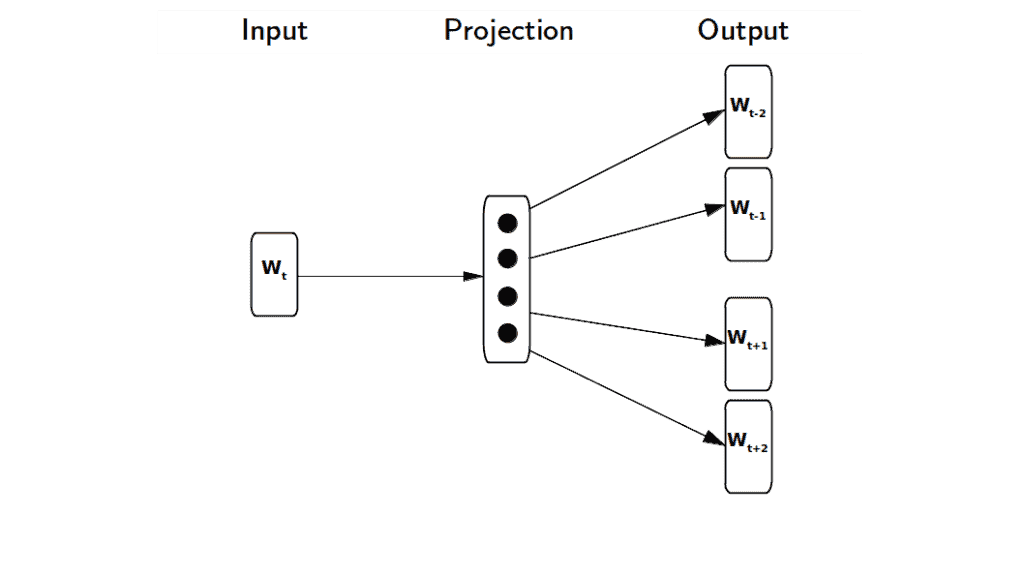
2. The Skip-Gram Model

The idea behind the word2vec models is that the words that appear in the same context (near each other) should have similar word vectors. Therefore, we should consider some notion of similarity in our objective when training the model. This is done using the dot product since when vectors are similar, their dot product is larger.

The Skip-gram model works in a way that, given an input, it predicts the surrounding or context words. Using this method, we can learn a hidden layer that we’ll use to calculate how probable a word is to occur as the context of the input:

3. The Computational Problem

Imagine that we have a sequence of words $w_1, ..., w_{n-1}, w_{T}$ as our training data. According to the original description of the Skip-gram model, published as a conference paper titled Distributed Representations of Words and Phrases and their Compositionality, the objective of this model is to maximize the average log-probability of the context words occurring around the input word over the entire vocabulary:

(1) $\begin{equation*} \frac{1}{T} \sum_{t=1}^{T} \sum_{-c \le j \le c, j \ne 0}^{} \textnormal{log } p(w_{t+j} | w_t) \end{equation*}$

where $T$ is all the words in the training data and $c$ is the training context window. The size of this window can affect the training accuracy and computational cost. Larger windows lead to higher accuracy as well as higher computational cost. One way to calculate the above probability is to use the softmax function:

(2) $\begin{equation*} p(w_{O}|w_{I}) = \frac{\textnormal{exp} (v^\prime_{w_{O}}^T v_{w_I})}{\sum_{w=1}^{W} \textnormal{exp } (v^\prime_{w}^T v_{w_I})} \end{equation*}$

where $v_w$ and $v^\prime_w$ are the vector representations of the word $w$ as the input and output, respectively. Also, $W$ is the number of words in the entire vocabulary.

The intuition is that words that appear in the same context will have similar vector representations. The numerator in the equation above will show this by assigning a larger value for similar words through the dot product of the two vectors. If the words do not occur in each other’s context, the representations will be different, and as a result, the numerator will be a small value.

However, the main problem comes up when we want to calculate the denominator, which is a normalizing factor that has to be computed over the entire vocabulary. Considering the fact the size of the vocabulary can reach hundreds of thousands or even several million words, the computation becomes intractable. This is where negative sampling comes into play and makes this computation feasible.

4. Negative Sampling

In a nutshell, by defining a new objective function, negative sampling aims at maximizing the similarity of the words in the same context and minimizing it when they occur in different contexts. However, instead of doing the minimization for all the words in the dictionary except for the context words, it randomly selects a handful of words ( $2 \le k \le 20$ ) depending on the training size and uses them to optimize the objective. We choose a larger $k$ for smaller datasets and vice versa.

The objective for the workaround that Mikolov et al. (2013) put forward is as follows:

(3) $\begin{equation*} \textnormal{log } \sigma (v^\prime_{w_O}^T v_{w_I}) + \sum_{i=1}^{k} \mathbb{E}_{w_i \sim P_n(w)} \left[ \textnormal{log } \sigma (-v^\prime_{w_i}^T v_{w_I}) \right] \end{equation*}$

where $\sigma$ is the sigmoid function. Also, $P_n(w)$ is called the noise distribution with the negative samples drawn from it. It’s calculated as the unigram distribution of the words to the power of $\frac{3}{4}$ which is a number that was calculated based on experimental results:

(4) $\begin{equation*} P_n(w) = \frac{U(w)^{\frac{3}{4}}}{Z} \end{equation*}$

where $Z$ is a normalization constant. Maximizing Formula 3 will result in maximizing the dot product in its first term and minimizing it in the second term. In other words, the words in the same context will be pushed to have more similar vector representations while the ones that are found in different contexts will be forced to have less similar word vectors.

As we can see from the Objective 3, the computation is done over the $\pmb{k}$ negative samples from the noise distribution, which is easily doable as opposed to computing the softmax over the entire vocabulary.

5. Deriving the Objective for Negative Sampling

Let’s assume that $(w, c)$ is a pair of words that appear near each other in the training data, with $w$ being a word and $c$ its context. Therefore, we can denote this by $p(D=1|w, c)$ , meaning that this pair came from the training data.

Consequently, the probability that the pair did not come from the training data will be $p(D=0|w, c) = 1 - p(D=1|w, c)$ . Denoting the trainable parameters of the probability distribution as $\theta$ and the notion of being out of training data as $D^\prime$ , we’ll have the following to optimize:

(5) $\begin{equation*} \textnormal{arg} \mathop{\textnormal{max}}_{\theta} \prod_{(w, c) \in D} p(D=1|w, c;\theta) \prod_{(w, c) \in D^\prime} p(D=0|w, c;\theta) \end{equation*}$

Substituting $p(D=0|w, c;\theta)$ with $1 - p(D=1|w, c;\theta)$ and converting the max of products to max of sum of logarithms, we’ll have:

(6) $\begin{equation*} \textnormal{arg} \mathop{\textnormal{max}}_{\theta} \sum_{(w, c) \in D} \textnormal{log } p(D=1|w, c;\theta) +\sum_{(w, c) \in D^\prime} \textnormal{log } (1 - p(D=1|w, c;\theta)) \end{equation*}$

We can compute $p(D=1|w, c;\theta)$ using the sigmoid function:

(7) $\begin{equation*} p(D=1|w, c;\theta) = \sigma(v_c.v_w) = \frac{1}{1 + e^{-v_c.v_w}} \end{equation*}$

where $v_w$ and $v_c$ are the vector representations of the main and context words, respectively. Therefore, Formula 6 becomes:

(8) $\begin{equation*} \textnormal{arg} \mathop{\textnormal{max}}_{\theta} \sum_{(w, c) \in D} \textnormal{log } \sigma(v_c.v_w) +\sum_{(w, c) \in D^\prime} \textnormal{log } (\sigma(-v_c . v_w)) \end{equation*}$

which is the same formula as Formula 3 summed over the entire corpus. For a more detailed derivation process, have a look at word2vec explained paper.

6. Conclusion

In this article, we described the Skip-gram model for training word vectors and learned about how negative sampling is used for this purpose. To put it simply, in order to reduce the computational cost of the softmax function which is done over the entire vocabulary, we can approximate this function by only drawing a few examples from the set of samples that do not appear in the context of the main word.

Full Archive

About Baeldung

Core Concepts

Operating Systems

Artificial Intelligence

Graph Theory

Latex