

Learn through the super-clean Baeldung Pro experience:
>> Membership and Baeldung Pro.
No ads, dark-mode and 6 months free of IntelliJ Idea Ultimate to start with.
Last updated: February 13, 2025
Learn through the super-clean Baeldung Pro experience:
>> Membership and Baeldung Pro.
No ads, dark-mode and 6 months free of IntelliJ Idea Ultimate to start with.
In this tutorial, we’ll talk about the two most popular types of layers in neural networks, the Convolutional (Conv) and the Fully-Connected (FC) layer. Both of them constitute the basis of almost every neural network for many tasks, from action recognition and language translation to speech recognition and cancer detection.
First, we’ll introduce the topic, and then we’ll define each type of layer separately. Finally, we’ll compare the two types of layers, illustrating their differences.
In an FC layer, all the neurons of the input are connected to every neuron of the output layer.
Specifically, let’s suppose that we have 7 input neurons ( ) and 5 output neurons (
 ). In an FC layer, we apply a weighted linear transformation to the input neurons and then pass the output through a non-linear activation function. So, the formula for computing the value of the output neurons in an FC layer is:
 where
where ![i \in [1, 5]](/wp-content/ql-cache/quicklatex.com-f760549697d359af2010eae29b57957a_l3.svg "Rendered by QuickLaTeX.com")
In the figure below, we can see what the neurons in the example FC layer look like:
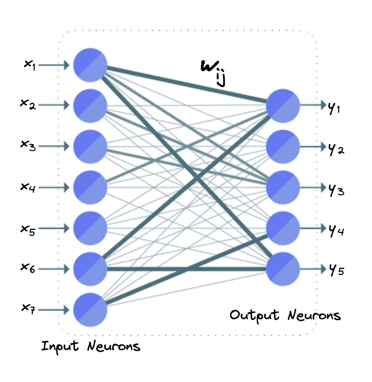
In an FC layer with  input and
  outputs, we have
  weights since each pair of input and output neurons correspond to a weight
  .
.
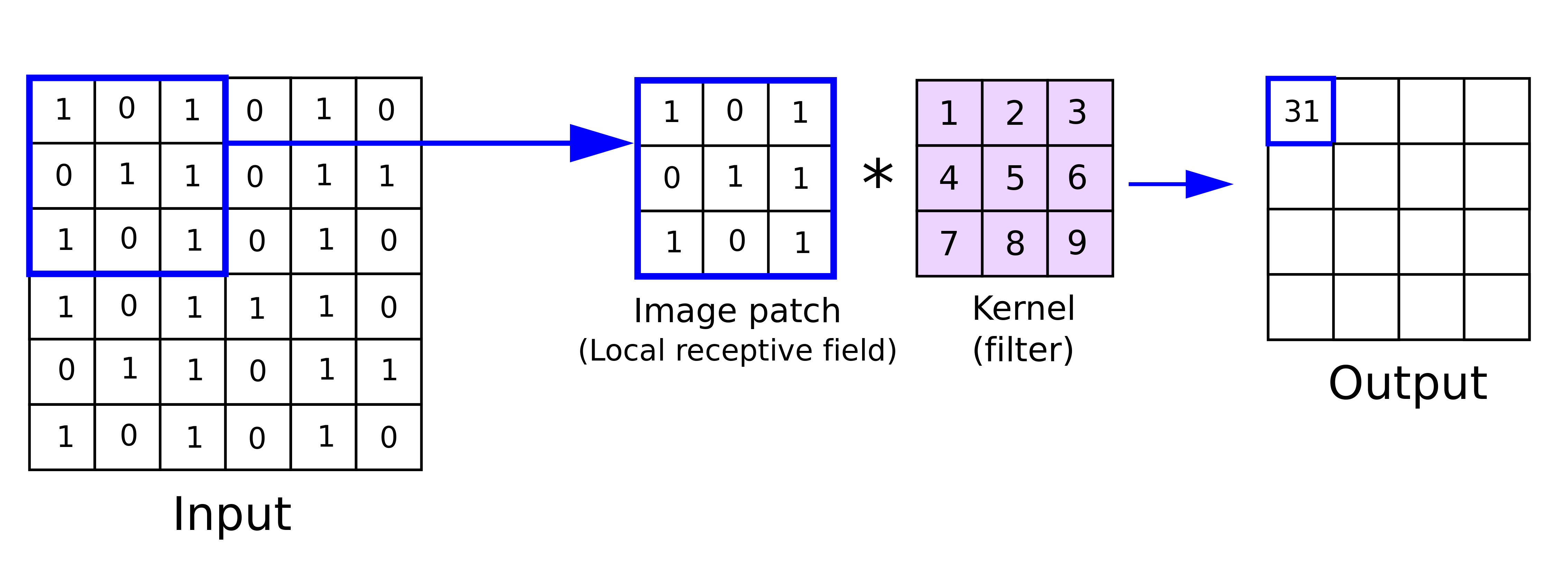
The basic operation of a convolutional layer is a convolution that is performed between an image and a kernel (or filter) that is equal to a square matrix. First, we perform element-wise multiplication between the pixels of the filter and the respective pixels of the image. Then, we sum up these multiplications into a single output value. The whole procedure is repeated for every pixel of the input image.
In the below image, we can see how convolution works between a  image and a
  filter. In the depicted step, we compute the convolution for the pixel (2, 2) of the image generating the below image patch:
In a convolutional layer, we perform convolution between the input neurons and some learnable filters, generating an output activation map of the filter. So, the number of weights is not dependent on the number of input neurons like in the FC layer. In a Conv layer, the number of weights is equal to the size of the kernel.
The basic difference between the two types of layers is the density of the connections. The FC layers are densely connected, meaning that every neuron in the output is connected to every input neuron. On the other hand, in a Conv layer, the neurons are not densely connected but are connected only to neighboring neurons within the width of the convolutional kernel. So, if the input is an image and the number of neurons is large, a Conv layer is more suitable.
A second main difference between them is weight sharing. In an FC layer, every output neuron is connected to every input neuron through a different weight  . However, in a Conv layer, the weights are shared among different neurons. This is another characteristic that enables Conv layers to be used in the case of a large number of neurons.
In this tutorial, we presented the Conv and the FC layer of a neural network. First, we introduced the terms, and then we discussed each layer separately, illustrating their differences.