Multi-Verse Optimizer | Baeldung on Computer Science

1. Overview

There are various optimization algorithms in computer science, and the Multi-Verse Optimization Algorithm (MVO) is one of them.

In this tutorial, we’ll take a look at what this algorithm means and what it does.

Then, we’ll go through the steps of the MVO algorithm. Finally, we’ll use a numerical example to demonstrate the solution to an optimization issue using MVO.

2. What Is the Multi-Verse Optimizer?

MVO is a population-based algorithm and a meta-heuristics algorithm based on the concepts of the multi-verse theory. As implied by the name, Seyedali Mirjalili introduced this approach for solving numerical optimization issues in 2015. The MVO algorithm is a physics-inspired technique, in particular, it’s inspired by the three main concepts of the multi-verse theory: white holes, black holes, and wormholes.

3. Multi-Verse Theory

The term multi-verse stands opposite to the universe and challenges the notion of uniqueness, which refers to the existence of additional worlds in addition to the one in which we all live. So, there might be duplicates, not only of objects but also of me, you, and everyone else.

In the multi-verse theory, multiple universes interact and may even collide with one another. The multi-verse approach also indicates that each world may have its own set of physical rules. The three fundamental concepts of the multi-verse theory are white holes, black holes, and wormholes.

3.1. White Holes

Although a white hole has never been observed in our world, the big bang may be regarded as a white hole and maybe the primary component in the formation of a universe. In addition, it is known in the cyclic model of the multi-verse theory that white holes (big bangs) are generated where parallel universes collide. Here’s an example of white holes:

3.2. Black Holes

Black holes, which have been discovered on several occasions, act radically differently from white wholes. With their tremendously strong gravitational pull, they attract everything, including light beams. The image below represents an example of black holes:

3.3. Wormholes

Wormholes are holes that link various sections of the universe. They operate as time/space travel tunnels in the multiverse approach. Items may move instantly between any two corners of a universe or even from one universe to another via these tunnels. Here’s an example of wormholes:

3.4. Rules of Universes in MVO

Let’s take a look at the principles that we apply, during the optimization process, to the universe of MVO:

The probability of having a white hole grows as the inflation rate increases.
The probability of having a black hole decreases as the inflation rate increases.
Universes with a higher inflation rate tend to send objects through white holes.
Universes with a lower inflation rate tend to receive more objects through black holes.
Regardless of the inflation rate, the objects in all universes may experience random movement towards the best universe via wormholes.

4. Mathematical Model of Multi-Verse Algorithm

Let’s divide the search procedure, which is used by a population-based algorithm, into two parts: exploration and exploitation. In order to explore search spaces through MVO, we use the ideas of a white hole and a black hole. Wormholes, on the other hand, help MVO exploit the search spaces.

Each solution is equivalent to a universe, and each variable in that world is an object. Furthermore, we apply an inflation rate to each solution that is proportional to the solution’s associated fitness function value.

4.1. Roulette Build Mechanism in MVO

We employ a roulette wheel mechanism to describe the mathematical model of the white and black hole tunnels, as well as the movement of objects across universes. The roulette wheel table, which is a game of chance, contains ${37}$ numbers ${(0-36)}$ . The color of number ${0}$ is green and the others colored with ${18}$ red & ${18}$ black. The graph below presents the roulette wheel:

So, we use the roulette mechanism to choose one universe among all for the white holes. At each iteration, we´ll sort the universe according to their fitness value (inflation rate) and select one using roulette.

4.2. Mathematical Model of Universe Selection

According to multi-verse theory, we have more than one universe:

${ U =}\begin{bmatrix} {x_{1}^1} & {x_{1}^2} & {.} & {.} & {.} & {x_{1}^d}\\ {x_{2}^1} & {x_{2}^2} & {.} & {.} & {.} & {x_{2}^d}\\ . & . & . & . & . & .\\ . & . & . & . & . & .\\ . & . & . & . & . & .\\ {x_{n}^1} & {x_{n}^2} & {.} & {.} & {.} & {x_{n}^d}\\ \end{bmatrix} \text{where d = number of parameters, n = total number of universes }$

The model below shows the mathematical model that we can use for the selection of one universe using the roulette wheel selection mechanism:

${U} = \left\{ \begin {array} {ll} {x_{k}^j} \text{ , } {r_{1} <} \text{ normalized inflation rate } ({U_{i}})\\ {x_{i}^j } \text{ , } {r_{1} \geq } \text{ normalized inflation rate } ({U_{i}}) \\ \end{array}$

Where ${x_{k}^j}$ represents the ${j^{th}}$ parameter of the ${k^{th}}$ universe selected by the roulette wheel mechanism, ${x_{i}^j }$ refers to the ${j^{th}}$ parameter of the ${i^{th}}$ universe, ${U_{i}}$ is the ${i^{th}}$ universe, and ${r_{1}$ is a random value in the interval ${[0,1]}$ .

Using this mechanism universes can exchange objects with each other without any disorganization.

4.3. Mathematical Model for Wormhole Tunnels

As we said before, the wormholes act as tunnels in between the black hole and white hole. So, let’s assume that each universe has wormholes to assure the exchange randomly of objects through space. The wormholes randomly change objects without consideration of their inflation rates. Let’s now suppose that wormhole tunnels are always established between a universe and the best universe (to provide local changes to each universe). Let’s discover the formulation of this mechanism:

${x_{i}^j} = \left\{ \begin {array} {ll} {\left\{ \begin {array} {ll} {X_{j} + TDR \times ((UpperBound_{j} - LowerBound_{j}) \times r_{4} + LowerBound_{j})} \text{ , } {r_{3} < 0.5} \\ {X_{j} - TDR \times ((UpperBound_{j} - LowerBound_{j}) \times r_{4} + LowerBound_{j})} \text{ , } {r_{3} \geq 0.5} \\ \end{array}} \text{ , } {r_{2} < WEP} \\ {x_{i}^j} \text{ , } {r_{2} \geq WEP} \\ \end{array}$

Where ${X_{j}}$ represents the ${j^{th}}$ variable of the fittest universe created, ${x_{i}^j }$ refers to the ${j^{th}}$ parameter of the ${i^{th}}$ universe, ${UpperBound} = \text{Maximum Limit}$ , ${LowerBound} = \text{Minimum Limit}$ , { ${r_{2}}$ , ${r_{3}}$ , ${r_{4}$ } ${=}$ random numbers in the interval ${[0,1]}$ , ${WEP} = \text{Wormhole Existance Probability}$ , and ${TDR} = \text{Travelling Distance Rate}$ .

The equations below represent the ${TDR}$ and the ${WEP}$ :

${WEP= min + l \times (\frac{max - min}{L})} \text{, where l = current iteration and L = maximum iteration}$

${TDR = 1 - \frac{l^{\frac{1}{p}}}{L^{\frac{1}{p}}}} \text{, where p = exploitation accuracy}$

5. Multi-Verse Algorithm

Let’s now take a look at the implementation of the MVO optimizer and its tile complexity.

5.1. Algorithm

The algorithm below represents the multi-verse optimizer:

algorithm MultiVerseOptimizer(U):
    // INPUT
    //    U = initial random universes
    // OUTPUT
    //    the Best Universe

    Initialize WER, TDR, and Best Universe
    SU <- Sorted universes
    NI <- Normalize inflation rate (fitness) of the universes

    while the end criterion is not satisfied:
        Evaluate the fitness of all universes

        for each universe (indexed by i):
            Update WEP and TDR
            Black hole index <- i

            for each object (indexed by j):
                r1 <- random([0, 1])

                if r1 < NI(U[i]):
                    White hole index <- RouletteWheelSelection(-NI)
                    U[Black hole index, j] <- SU[White hole index, j]

                r2 <- random([0, 1])

                if r2 < WEP:
                    r3 <- random([0, 1])
                    r4 <- random([0, 1])

                    if r3 < 0.5:
                        U[i, j] <- Best Universe[j] + TDR * ((ub[j] - lb[j]) * r4
                          + lb[j])
                    else:
                        U[i, j] <- Best Universe[j] - TDR * ((ub[j] - lb[j]) * r4
                          + lb[j])

    return Best Universe

As we can see in the algorithm, the population size (number of universes) and the maximum number of iterations are needed as inputs in order to get the Best Universe and its Fitness value as the output of the algorithm.

We start by initializing the parameters { ${r_1, r_2, r_3, r_4}$ }, { ${WER, TDR,} \text{ Best Universe,} \text{ Black hole index (i), } {SU, NI}$ } and the population size ${U_n (n = 1, 2, 3, ..., N)$ }. Then, we evaluate each solution by calculating its value using the fitness function. After evaluating each solution in the population, we assign the best solution according to its value. Afterward, we update the parameters ${WER, TDR}$ .

In order to select one universe among N, we use the roulette wheel selection mechanisms as a white hole. Then, we use a wormhole as a tunnel for object exchange between different universes. We repeat the overall operations until the stopping criteria are matched, which means we will check the current iteration until we reach the maximum number of iterations to return the best global solution.

5.2. Time Complexity of MVO

It is worth noting that the time complexity of the multi-verse algorithm is generally related to the number of iterations ( ${l}$ ), the number of universes ( ${n}$ ), and the number of objects ( ${d}$ ). So, the equation below represents the time complexity of this algorithm:

${{O}(MVO) = {O}(l(O(QuickSort) + n \times d \times ({O}(Roulette Wheel))))}$

In more detail, we employ the QuickSort algorithm in every iteration, which has the complexity of ${O(n^2)}$ in the worst case. In addition, we use the roulette wheel mechanism for every variable in every universe over the iterations, which has the complexity of ${O(log(n))}$ in the worst case. Let’s reconstruct the time complexity of the multi-verse algorithm using the complexity of Quick Sort and roulette wheel mechanism:

$\boldsymbol{{O}(MVO) = {O}(l(n^2 + n \times d \times log(n)))}$

6. Numerical Example of Multi-Verse Algorithm

To understand the multi-verse optimizer algorithm, we use a numerical example.

6.1. Initialization

Firstly, we randomly initialize the population size (total number of universes) ${N = 4}$ . Afterward, we initialize all the parameters using a random set of values:

$\left\{ \begin {array} {llllll} { SU} = \text{ Sorted Universes} } \\ { NI = \text{Normalized Inflation rate} } \\ { i = \text{Black Hole Index }} \\ { r_1, r_2, r_3, r_4 = \text{ random numbers in [0, 1] }} \\ { \text{Population size (total number of universes)}} \\ { \text{WEP, TDR} } \\ \end{array}$

Here’s the initial position for the four universes ( ${N = 4}$ ):

Sr. No	1	2	3	4	5
1.	-70.8536	85.1716	-43.5590	-26.9935	-33.5764
2.	17.0087	-1.4723	95.1915	-38.1701	79.4960
3.	-85.3277	30.9766	-92.7149	-75.8175	-0.0702
4.	64.4652	78.0247	-34.7511	83.1531	23.0576

Sr. No	6	7	8	9	10
1.	39.6508	-32.0028	-90.4425	-77.1940	-72.7985
2.	-94.1335	69.3422	-89.2045	59.2491	57.7783
3.	5.5765	-50.7861	-95.8764	23.5701	-81.5203
4.	-93.5854	16.2983	36.2957	-85.9573	-52.4262

6.2. Compute the Fitness Value

Here’s the fitness function in order to compute the fitness value for each universe and select the Best Universe:

$Fitness Function= 4 \times {X(1)^2} - 2.1 \times {X(1)^4} + \frac{1}{3} \times {X(1)^6} + {X(1)} \times {X(2)} - 4 \times {X(2)^2} + 4 \times {X(2)^4}$

Let’s calculate the fitness value for each universe in the current population using the fitness function:

Sr. No	Fitness Value
1.	3.8063 * e⁴
2.	4.5605 * e⁴
3.	4.1588 * e⁴
4.	3.9376 * e⁴

6.3. Optimal Solution and Update Parameters

After calculating all the fitness values (inflation rate of each universe), we select the optimal solution (Best Universe) among all. The optimal solution is the one that has the smallest fitness value across all universes. As a result, ${Fitness = 3.8063 \times e^4}$ is the best solution for the first iteration. Let’s move forward to update the parameters of ${ \text{WEP}}$ and $\text{TDR}$ for each universe:

$\left\{ \begin {array} {ll} { WEP} = 0.2080 } \\ { TDR = 0.5358 } \\ \end{array}$

6.4. Selection of Universe

We need to select one universe among N by using the roulette wheel selection mechanism as a white hole based on the mathematical model below:

Where ${r_1 = 0.8558}$ is chosen at random from the interval ${[0, 1]}$ . So, to elect one among all for the white hole, we apply the two rules below:

The universe with a higher inflation rate is considered to have a white hole.
The universe with a low inflation rate is considered to have a black hole.

In other words, the fitness value with the highest value represents the only white hole. At each iteration, we’ll sort the universe according to the fitness value. The table below depicts the choosing of one white hole as the second universe, while the other universes are black holes:

Sr. No	Fitness Value
1.	3.8063 * e⁴
2.	4.5605 * e⁴
3.	4.1588 * e⁴
4.	3.9376 * e⁴

6.5. Wormhole Tunnel

Let’s now use a transportation medium to move objects from the universe with a white hole to the universe with a black hole. In this case, we use the wormhole as the tunnel to exchange objects between different universes:

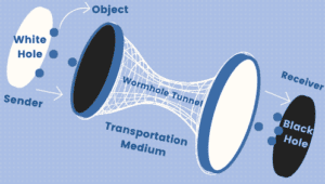
So, the wormholes act as time/space travel tunnels between different universes based on the mathematical model below:

Where ${\begin{pmatrix} \begin {array} {ll} {r_2 = 0.6708} \\ {r_3 = 0.5236} \\ \end{array} \end{pmatrix}}$ are chosen at random from the interval ${[0, 1]}$ . We have ${(r_2 = 0.6708) > (WEP= 0.2080)}$ then ${{x_{i}^j} = {x_{i}^j}}$ . This means the best universe formed with the ${\text{fitness value} = 3.8063 \times e^4}$ .

6.6. Update Best Universe

Let’s now check the maximum iteration and the current iteration then we repeat the steps above until reaching the criteria. After the repetition of the loop, we got the best optimum value ${= 0.0049209}$ . Then, we display ${0.0049209}$ as the best universe.

7. Conclusion

In this article, we discussed the multi-verse optimization algorithm using a numerical example to unlock its mechanism. This algorithm searches for the best universe, which represents the best solution to a problem based on the multi-verse theory. We introduced this algorithm because it’s highly effective in solving global unconstrained and constrained optimization issues.

Core Concepts

Operating Systems

Artificial Intelligence

Graph Theory

Latex

Full Archive

About Baeldung