

Yes, we're now running our only Summer Sale. All Courses are 30% off until 20th July, 2026:
Learn through the super-clean Baeldung Pro experience:
>> Membership and Baeldung Pro.
No ads, dark-mode and 6 months free of IntelliJ Idea Ultimate to start with.
1. Overview
In this tutorial, we’ll talk about motion field and optical flow, two important concepts in computer vision. We’ll explain their mathematical definitions and provide examples to highlight their differences.
2. Motion Field
In computer vision, the motion field represents the 3D motion as it is projected onto an image plane. The primary goal of object tracking is to estimate the motion field.
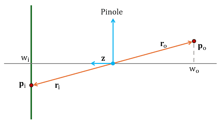
Let’s consider a point  in a three-dimensional scene at position
  . We consider a reference system whose origin is fixed at the camera’s pinhole. The point
  located at
  is the projection of the point onto the image plane. The following figure represents this scenario:
The point moves in the three-dimensional scene with velocity  . In a small time interval
  , the point moves to a new location
  . Hence, the velocity of the scene point is defined as:
(1) 
Similarly, the image point moves with velocity:
(2) 
The following figure shows the displacement of the physical point and the corresponding one on the image plane:
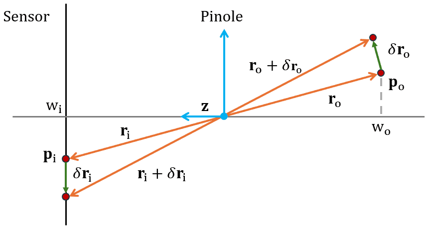
We want to determine the relationship between image velocity and scene velocity. We observe that the triangles X and Y are similar, therefore we can write:
(3) 
where  is the focal length and
  is a unit vector collinear to the optical axis. By substituting r_i from eq. (3) in eq (2), we can rewrite the image velocity by applying the quotient rule of the derivatives:
(4) 
this expression can be furthermore simplified using the cross-product:
(5) 
The latter equation relates the velocity and position of the point with the corresponding velocity in the image  , representing the motion field. The latter cannot be measured directly. In object tracking, the motion field can be measured in some particular condition by estimating the optical flow.
3. Optical Flow
The optical flow is the apparent motion of brightness patterns in the image. Let’s consider a sequence of images captured by a camera as a video. Algorithms for optical flow estimation analyze the pixel intensity patterns between frames to determine their displacement. By observing how these intensities change, the algorithm infers the motion of objects in the scene.
For example, the following animation shows two consecutive video frames:
We can see that several brightness patterns are moving between the frames. Optical flow is the motion of each brightness pattern. Conversely, the motion field represents the motion of each pixel in the frame.
The Lucas-Kanade algorithm is the most popular algorithm for computing the optical flow. This method assumes that motion is constant within a local neighborhood and computes optical flow using spatial gradients. It’s efficient and works well for small motion.
4. Examples
Ideally, the optical flow would be the same as the motion field. Unfortunately, this is not always true, and we will show some particular cases here.
Let’s consider a rotating sphere and a fixed light:
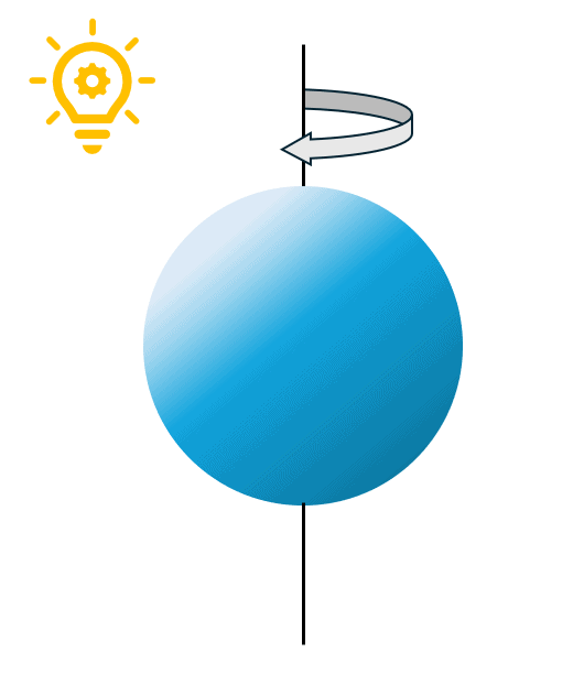
The sphere is made of a single material that spins around the vertical axis, passing through its center. Since the points of the sphere are moving, there is a non-zero motion field. Conversely, there is no optical flow because all the image frames acquired by a stationary camera are identical.
Let’s now consider the same sphere but fixed and the light source moving around it:
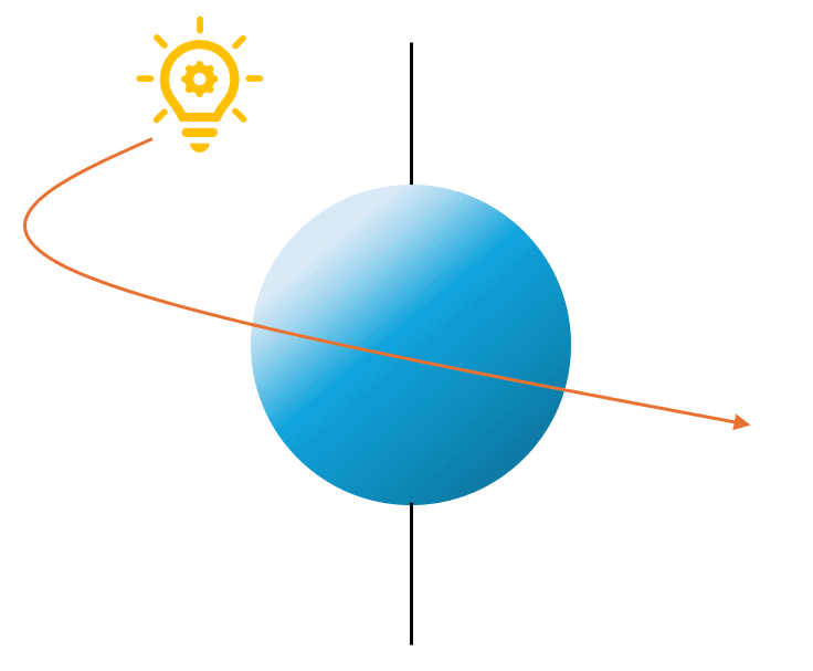
In this case, we observe a shading change and brightness patterns moving in the images as the light source moves. Hence, there is a non-zero optical flow but no motion field.
Hence, we understand that optical flow does not always correspond to the motion field. In some cases, the optical flow is different from the motion field.
An interesting example is the barber-pole illusion represented here:

The barber pole rotates along the vertical axis; hence, all points on the cylinder move horizontally. Conversely, brightness patterns move in a vertical direction. The following figure represents the barber’s pole’s optical flow and motion field:
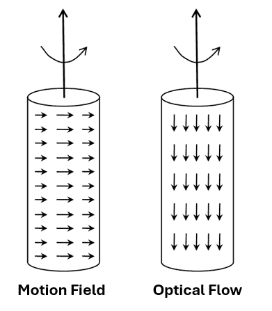
Hence, we observe both optical flow and motion field in this case, but they don’t correspond.
5. Conclusion
In this article, we reviewed the motion field and the optical flow, two fundamental notions in computer vision. First, we explained their definition, and finally, we illustrated several examples to highlight their differences.