What Is Gradient Orientation and Gradient Magnitude?

1. Introduction

Gradient orientation and gradient magnitude are fundamental concepts in the field of computer vision and image processing. Moreover, these concepts are used to extract information from digital images and enable a range of applications such as object recognition, image segmentation, and edge detection.

In this tutorial, we’ll discuss the basics of gradient orientation and gradient magnitude.

2. What Is Gradient Orientation?

First, let’s discuss the definition of the gradient orientation. Gradient orientation refers to the direction of an image’s maximum change in intensity.

In particular, there’re several ways to perform calculations. However, one common approach is to use the central difference method. Furthermore, this involves calculating the partial derivatives of an image with respect to the $x$ and $y$ directions.

Additionally, the partial derivative in the $x$ direction represents the rate of change in the horizontal direction. In contrast, the partial derivative in the $y$ direction represents the rate of change in the vertical direction.

Therefore, the gradient orientation is computed using the following equation:

$\theta = Arctan(\frac{G_y}{G_x})$

where $Gy$ and $Gx$ are the partial derivatives in the $y$ and $x$ directions, respectively, and $\theta$ is the gradient orientation. Moreover, the gradient orientation is typically measured in radians.

Additionally, the gradient orientation is invariant to the rotation of the image. Hence, the same object in an image will have the same gradient orientation regardless of its orientation.

3. What Is Gradient Magnitude?

Now, let’s discuss the definition of the gradient magnitude. Gradient magnitude refers to the strength of an image’s intensity change.

Typically, there’re multiple calculation methods. However, based on the simple central difference method, it’s computed by taking the square root of the sum of the squares of the partial derivatives in the $x$ and $y$ directions.

Therefore, the gradient magnitude is computed using the following equation:

$|G|=\sqrt{{G_x^2+G_y^2}}$

where $Gx$ and $Gy$ are the partial derivatives in the $x$ and $y$ directions, respectively, and $|G|$ is the gradient magnitude.

Additionally, the gradient magnitude can be visualized as a grayscale image, where the intensity of each pixel represents the strength of the gradient at that location.

Moreover, high gradient magnitude values usually indicate edges in an image. However, in areas with high noise levels, the gradient magnitude can also be high, even if there is no meaningful change in intensity.

4. An Example

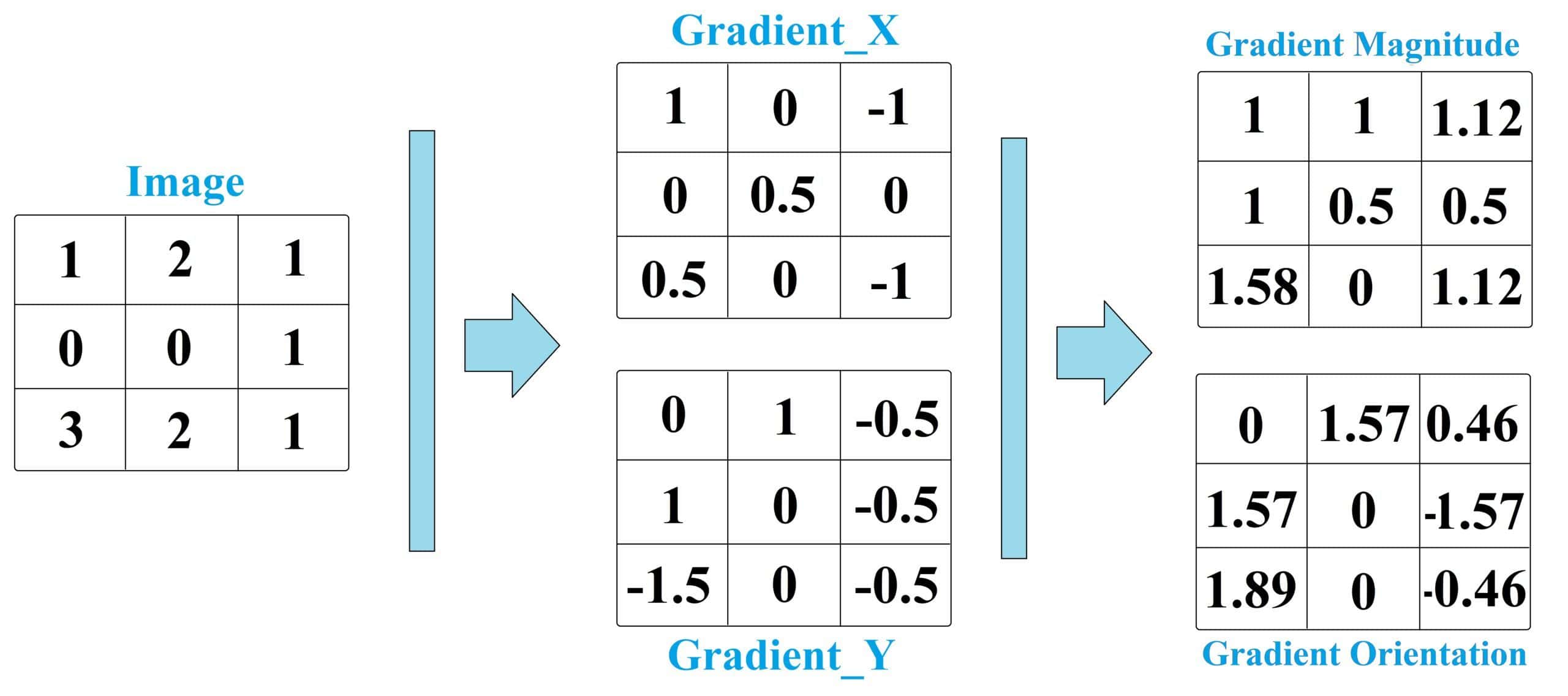
Let’s say we have a grayscale image with pixel values represented by the following matrix:

$Image =\left[\begin{array}{ccc} 1 & 2 & 1 \\ 0 & 0 & 1 \\ 3 & 2 & 1 \end{array}\right]$

Hence, we can calculate the gradient in the $x$ -direction using the central difference method as follows:

$\operatorname{gradient}_x (i, j)=\frac{(f(i, j+1)-f(i, j-1))}{2}$

Moreover, note that if $f(x,y)$ refers to an element beyond the matrix, its value would be zero. For instance, in the above example, $f(i,4)$ or $f(i,0)$ have zero values since $j$ =1, 2, and 3 are the only existing columns of the matrix.

Finally, we have:

$gradient_x =\left[\begin{array}{ccc} \frac{2-0}{2} & \frac{1-1}{2} & \frac{0-2}{2}\\ \\ \frac{0-0}{2} & \frac{1-0}{2} & \frac{0-0}{2}\\ \\ \frac{2-0}{2} & \frac{1-3}{2} & \frac{0-2}{2} \end{array}\right] =\left[\begin{array}{ccc} 1 & 0 & -1 \\ 0 & 0.5 & 0 \\ 1 & -1 & -1 \end{array}\right]$

Similarly, we can calculate the gradient in the $y$ -direction as follows:

$\operatorname{gradient}_y (i, j)=\frac{(f(i+1, j)-f(i-1, j))}{2}$

Again, note that if $f(x,y)$ refers to an element beyond the matrix, its value would be zero. For instance, in the above example, $f(4,j)$ or $f(0,j)$ have zero values since $i$ =1, 2, and 3 are the only existing rows of the matrix.

Thus, we have:

$gradient_y = \left[\begin{array}{ccc} \frac{0-0}{2} & \frac{2-0}{2} & \frac{1-0}{2}\\ \\ \frac{3-1}{2} & \frac{2-2}{2} & \frac{1-1}{2}\\ \\ \frac{0-0}{2} & \frac{0-0}{2} & \frac{0-1}{2} \end{array}\right] =\left[\begin{array}{ccc} 0 & 1 & 0.5 \\ 1 & 0 & 0 \\ 0 & 0 & -0.5 \end{array}\right]$

Finally, once we have the gradient in the directions for $x$ and $y$ , we can calculate the gradient magnitude and orientation using the formulas mentioned in the previous section.

$Gradient Magnitude =\left[\begin{array}{ccc} 1 & 1 & 1.118 \\ 1 & 0.5 & 0.5 \\ 1.581 & 0 & 1.118 \end{array}\right]$

Additionally, note the values for gradient orientation are calculated based on radians. So, for example, 1.57 simply means 90 degrees.

$Gradient Orientation =\left[\begin{array}{ccc} 0 & 1.57 & 0.46 \\ 1.57 & 0 & -1.57 \\ 1.892 & 0 & -0.464 \end{array}\right]$

Furthermore, if a pixel’s gradients in both $x$ and $y$ direction are zero, then the gradient orientation cannot be calculated using the mentioned formula. Thus, this is because dividing by zero is undefined, and the formula requires a non-zero denominator.

In such cases, the gradient orientation is usually set to 0 or 180 degrees, depending on the convention being used. Hence, we set 0 for the pixel at the location of (3,2):

5. Alternative Methods of Calculation

In this article, we used the central difference method. However, several other methods can be used to calculate the gradient magnitude and orientation, depending on the specific application and the computational resources available. Therefore, the choice of method will depend on the specific application and the tradeoff between accuracy and computational resources.

Therefore, let’s discuss some additional methods in the following subsections.

5.1. Sobel Operator

The Sobel operator is a popular edge detection filter that calculates the gradient magnitude and orientation by convolving the image with a small kernel. Hence, this method is more accurate than the central difference but may be more computationally expensive.

5.2. Prewitt Operator

The Prewitt operator is similar to the Sobel operator but uses a slightly different kernel. Like the Sobel operator, it’s more accurate than the central difference method but may be more computationally expensive.

5.3. Laplacian of Gaussian (LoG)

The LoG method involves convolving the image with a Gaussian filter to smooth out noise and then taking the Laplacian of the resulting smoothed image. Therefore, this method is more complex than the previous methods but can be more accurate, especially for detecting small details in the image.

5.4. Canny Edge Detection

The Canny edge detection algorithm is a multi-stage process that involves smoothing the image, calculating the gradient magnitude and orientation using the Sobel operator, and applying non-maximum suppression to thin the edges. Finally, we apply hysteresis thresholding to identify strong edges. Hence, this method is considered one of the most accurate and robust edge detection techniques.

6. Applications of Gradient Orientation and Gradient Magnitude

Gradient orientation and gradient magnitude are widely used in computer vision and image processing applications. Here are some of the applications:

Object detection: Object detection is one of the most important applications of gradient orientation and magnitude. In object detection, a trained model is used to identify objects in an image. Additionally, the model uses gradient orientation and gradient magnitude to identify regions of the image likely to contain objects of interest
Edge detection: Edge detection is another important application of gradient orientation and magnitude. Moreover, edge detection is used to identify boundaries between regions of an image that have different intensities. Additionally, gradient magnitude is used to identify regions of the image with a significant change in intensity, while gradient orientation is used to identify the direction of the edge
Image segmentation: Image segmentation divides an image into multiple regions or segments. Moreover, gradient orientation and gradient magnitude can segment an image by identifying regions with similar gradient properties. For example, regions with similar gradient orientation and magnitude may belong to the same object in the image
Texture analysis: Texture analysis is the process of identifying and characterizing the patterns in an image. Therefore, gradient orientation and gradient magnitude can be used to identify and quantify the texture in an image. Additionally, analyzing the gradient orientation and magnitude at different locations in an image makes it possible to identify the patterns that make up the texture

7. Conclusion

In this article, we explained gradient orientation and magnitude and their applications. Understanding these concepts is crucial for developing accurate algorithms for analyzing digital images.

Core Concepts

Operating Systems

Neural Networks

Graph Theory

Latex

Full Archive

About Baeldung