

Learn through the super-clean Baeldung Pro experience:
>> Membership and Baeldung Pro.
No ads, dark-mode and 6 months free of IntelliJ Idea Ultimate to start with.
Learn through the super-clean Baeldung Pro experience:
>> Membership and Baeldung Pro.
No ads, dark-mode and 6 months free of IntelliJ Idea Ultimate to start with.
Very often when working with video streams, it’s necessary to characterize and quantify the motions of the objects moving in the video. This can be done by estimating the optical flow between two frames.
In this tutorial, we will explore what optical flow is and how to calculate it.
The concept of optical flow was actually first introduced in the field of psychology. In the 1940s, an American psychologist named James J. Gibson used the term to describe the visual stimulus provided to animals moving through the world.
Like animals, we’re often very interested in the part that is moving in a scene. But in a video, a computer sees the world in numbers. That is why in computer vision, the term optical flow refers to a vector field between two images that describe how the pixels of an object in the first image change in relation to the second image.
Since video streams are widely used, optical flow is very important for applications like camera image stabilization, traffic control, and autonomous navigation.
Let’s look at an example:
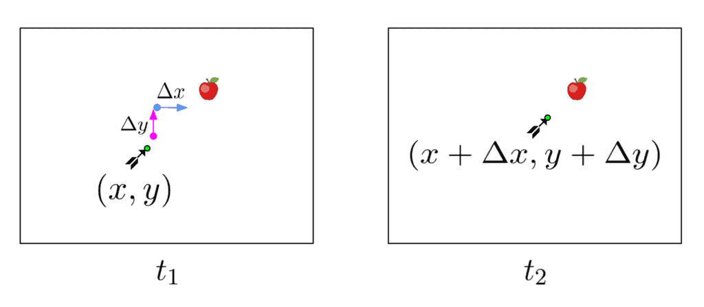
Here we have two video frames of an arrow approaching an apple. Consider a pixel point inside the arrow object containing the very tip of the arrow. Between the two frames, it has traveled some pixels on the  -axis and some on the
  -axis. If we label the distances as
  and
and  accordingly, the so-called optical flow corresponding to the arrow tip will be
  . This is what we want to measure.
Estimating the optical flow, however, turns out to be a difficult task. One obvious problem is that we have no way of finding the corresponding pixels of the objects between the two images, meaning we’re not sure where exactly the arrow lies.
For a solution to be possible we have to assume that the intensity or brightness of all the image pixels stays the same. If the object changed its brightness as it moves, the problem becomes extremely complex. This allows us to associate the pixels and put forth an equation:
A point at location  with intensity
  will have moved by
  ,
, and
and  between the two image frames:
![\[I(x,y,t) = I(x+\Delta x, y + \Delta y, t + \Delta t)\]](/wp-content/ql-cache/quicklatex.com-066258a489569e9ec6e0d2e540accb59_l3.svg "Rendered by QuickLaTeX.com")
Another assumption that has to be made is that the pixel displacement and difference in time  between the two frames are sufficiently small. This is needed for us to come up with an approximate equation, that hopefully can be solved.
Based on this assumption we can expand the equation using the Taylor series:
![\[{\displaystyle I(x+\Delta x,y+\Delta y,t+\Delta t)=I(x,y,t)+{\frac {\partial I}{\partial x}}\,\Delta x+{\frac {\partial I}{\partial y}}\,\Delta y+{\frac {\partial I}{\partial t}}\,\Delta t+ \text{higher-order terms}{}}\]](/wp-content/ql-cache/quicklatex.com-ac524881cb877ef02e579f954da34068_l3.svg "Rendered by QuickLaTeX.com")
If we consider just the linear terms and discard the higher-order terms we get:

which can be then divided by  :
:
![\[\frac{\partial I}{\partial x}V_x+\frac{\partial I}{\partial y}V_y+\frac{\partial I}{\partial t} = 0\]](/wp-content/ql-cache/quicklatex.com-bfcfae5c911d44687c5cef345b65d0fa_l3.svg "Rendered by QuickLaTeX.com")
where  are the and components of the optical flow
  .
.
The resulting equation unfortunately has two unknowns and cannot be solved. This is known as the aperture problem. Geometrically it can be interpreted as the inability to grasp the real direction of an object if you only see a sliver limited by some aperture.
To overcome this, a more constrained set of equations are needed. That is why researchers have used algorithms like the Lucas-Kanade method to estimate the optical flow over image patches instead of individual pixels. Other approaches would consider only edges on the image.
Recently, however, algorithms based on the deep learning paradigm have gained traction and are evaluated as state-of-the-art on many open datasets. Every year researchers come up with new neural network architectures and build upon recent advances in machine learning and computer vision.
In this article, we learned about optical flow and what applications it has through a simplified example. We also managed to dabble a bit into the math behind it and introduced the problems that come up when trying to estimate it. Problems that fortunately didn’t stop researchers from coming up with new ways to tackle them and improve the field of computer vision.