

Learn through the super-clean Baeldung Pro experience:
>> Membership and Baeldung Pro.
No ads, dark-mode and 6 months free of IntelliJ Idea Ultimate to start with.
Learn through the super-clean Baeldung Pro experience:
>> Membership and Baeldung Pro.
No ads, dark-mode and 6 months free of IntelliJ Idea Ultimate to start with.
In this tutorial, we’ll discuss how to implement the merge sort algorithm using an iterative algorithm. First of all, we’ll explain the merge sort algorithm and the recursive version of it.
After that, we’ll discuss the iterative approach of this algorithm. Also, we’ll present a simple example to clarify the idea.
Finally, we’ll present a comparison between the iterative and the recursive algorithms and when to use each one.
As we know, the merge sort algorithm is an efficient sorting algorithm that enables us to sort an array within  time complexity, where
  is the number of values.
Usually, we find that the recursive approach more widespread. Thus, let’s quickly remember the steps of the recursive algorithm so that it’s easier for us to understand the iterative one later. The recursive version is based on the divide and conquers strategy:
As we showed in the recursive version, we divided the input into two halves. This process continued until we got each element of the array alone. Then, we merged the sorted parts from bottom to top until we get the complete result containing all the values sorted.
As usual, when we’re trying to think about moving from a recursive version to an iterative one, we have to think in the opposite way of the recursion. Let’s list a few thoughts that will help us implement the iterative approach:
Now, we can jump into the implementation. However, to simplify the algorithm, we’ll first implement a function responsible for merging two adjacent parts. After that, we’ll see how to implement the complete algorithm based on the merge function.
Let’s implement a simple function that merges two sorted parts and returns the merged sorted array, which contains all elements in the first and second parts.
Take a look at the implementation:
algorithm Merge(A, L1, R1, L2, R2):
    // INPUT
    //     A = the array to be sorted
    //     L1 = the start of the first part
    //     R1 = the end of the first part
    //     L2 = the start of the second part
    //     R2 = the end of the second part
    // OUTPUT
    //     Returns the merged sorted array

    temp <- []
    index <- 0
    while L1 <= R1 and L2 <= R2:
        if A[L1] <= A[L2]:
            temp[index] <- A[L1]
            index <- index + 1
            L1 <- L1 + 1
        else:
            temp[index] <- A[L2]
            index <- index + 1
            L2 <- L2 + 1

    while L1 <= R1:
        temp[index] <- A[L1]
        index <- index + 1
        L1 <- L1 + 1

    while L2 <= R2:
        temp[index] <- A[L2]
        index <- index + 1
        L2 <- L2 + 1

    return temp
In the merging function, we use three  loops. The first one is to iterate over the two parts together. In each step, we take the smaller value from both parts and store it inside the
  array that will hold the final answer.
Once we add the value to the resulting , we move  one step forward. The variable points to the index that should hold the next value to be added to .
In the second loop, we iterate over the remaining elements from the first part. We store each value inside . In the third loop, we perform a similar operation to the second loop. However, here we iterate over the remaining elements from the second part.
The second and third loops are because after the first loop ends, we might have remaining elements in one of the parts. Since all of these values are larger than the added ones, we should add them to the resulting answer.
The complexity of the merge function is  , where
  is the length of the first part, and
  is the length of the second one.
Note that the complexity of this function is linear in terms of the length of the passed parts. However, it’s not linear compared to the full array  because we might call the function to handle a small part of it.
Now let’s use the merge function to implement the merge sort iterative approach.
Take a look at the implementation:
algorithm IterativeMergeSort(A, n):
    // INPUT
    //     A = the array
    //     n = the size of the array
    // OUTPUT
    //     sorted array

    len <- 1
    while len < n:
        i <- 0
        while i < n:
            L1 <- i
            R1 <- i + len - 1
            L2 <- i + len
            R2 <- i + 2 * len - 1

            if L2 >= n:
                break

            if R2 >= n:
                R2 <- n - 1

            temp <- Merge(A, L1, R1, L2, R2)
            for j <- 0 to R2 - L1 + 1:
                A[i + j] <- temp[j]

            i <- i + 2 * len

        len <- 2 * len

    return A
Firstly, we start  from
from  that indicates the size of each part the algorithm handles at this step.
In each step, we iterate over all parts of size and calculated the beginning and end of each two adjacent parts. Once we determined both parts, we merged them using the  function defined in algorithm 1.
Note that we handled two special cases. The first one is if  reaches the outside of the array, while the second one is when
  reaches the outside. The reason for these cases is that the last part may contain less than elements. Therefore, we adjust its size so that it doesn’t exceed .
After the merging ends, we copy the elements from into their respective places in .
Note that in each step, we doubled the length of a single part . The reason is that we merged two parts of length . So, for the next step, we know that all parts of the size  are now sorted.
Finally, we return the sorted .
The complexity of the iterative approach is , where is the length of the array. The reason is that, in the first loop, we double the value in each step. So, this is  . Also, in each step, we iterate over each element inside the array twice and call the function for the complete array in total. Thus, this is
  .
.
Let’s take an example to understand the iterative version more clearly. Suppose we have an array as follows:
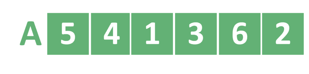
Let’s apply the iterative algorithm to .
In the first step, we’ll be merging the  element with the
  one. As a result, we’ll get a new sorted part which contains the first two values. Since the is smaller than the , we’ll swap both of them.
Similarly, we perform this operation for the  and
and  elements. However, in this case, they’re already sorted, and we keep their order. We continue this operation for the
  and
and  values as well.
After these steps, will have its parts of size 2 sorted as follows:
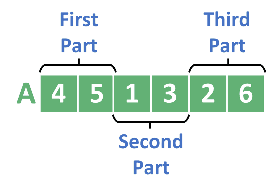
In the second step, the becomes 2. Hence, we have three parts. Each of these parts contains two elements. Similarly to the previous steps, we have to merge the first and the second parts. Thus, we get a new part that contains the first four values. For the third part, we just skip it because it was sorted in the previous step, and we don’t have a fourth part of merging it with.
Take a look at the result after these steps:
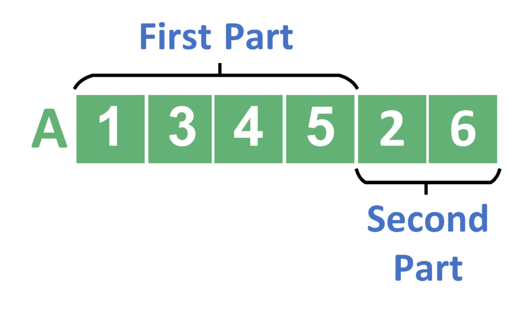
In the last step, the becomes 4, and we have two parts. The first one contains four elements, whereas the second one contains two. We call the merging function for these parts.
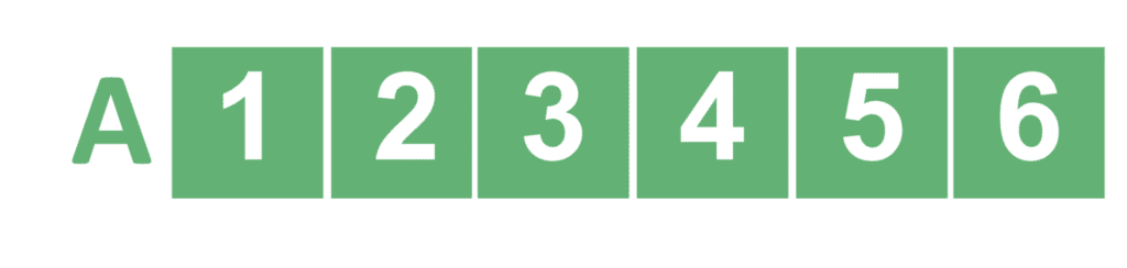
After the merging ends, we get the final sorted answer:
As usual, recursion reduces the size of the code, and it’s easier to think about and implement. On the other hand, it takes more memory because it uses the stack memory which is slow in execution.
For that, we prefer to use the iterative algorithm because of its speed and memory saving. However, if we don’t care about execution time and memory as if we have a small array, for example, we can use a recursive version.
In this tutorial, we explained how to implement the merge sort algorithm using an iterative approach. Firstly, we discussed the merge sort algorithm using the recursive version of the algorithm.
Then, we discussed the iterative version of this algorithm. Also, we explained the reason behind its complexity.
After that, we provided a simple example to clarify the idea well.
Finally, we presented a comparison between the iterative and the recursive algorithms and showed the best practice of using each of them.