Merging Two Binary Search Trees

1. Overview

A binary search tree (BST) is a fundamental data structure and is a type of binary tree where the value of a left node is less than the parent and the value of a right node is greater than the parent.

In this tutorial, we’re going to learn about two algorithms that can be used to merge two binary search trees. Also, we’ll discuss the complexity a.k.a Big O of these algorithms. The complexity of an algorithm is extremely important as it measures the amount of time and space required to run the algorithm.

There are two binary search trees (BST1 and BST2) in the following image. The merging of these two trees will produce merged BST as shown below:

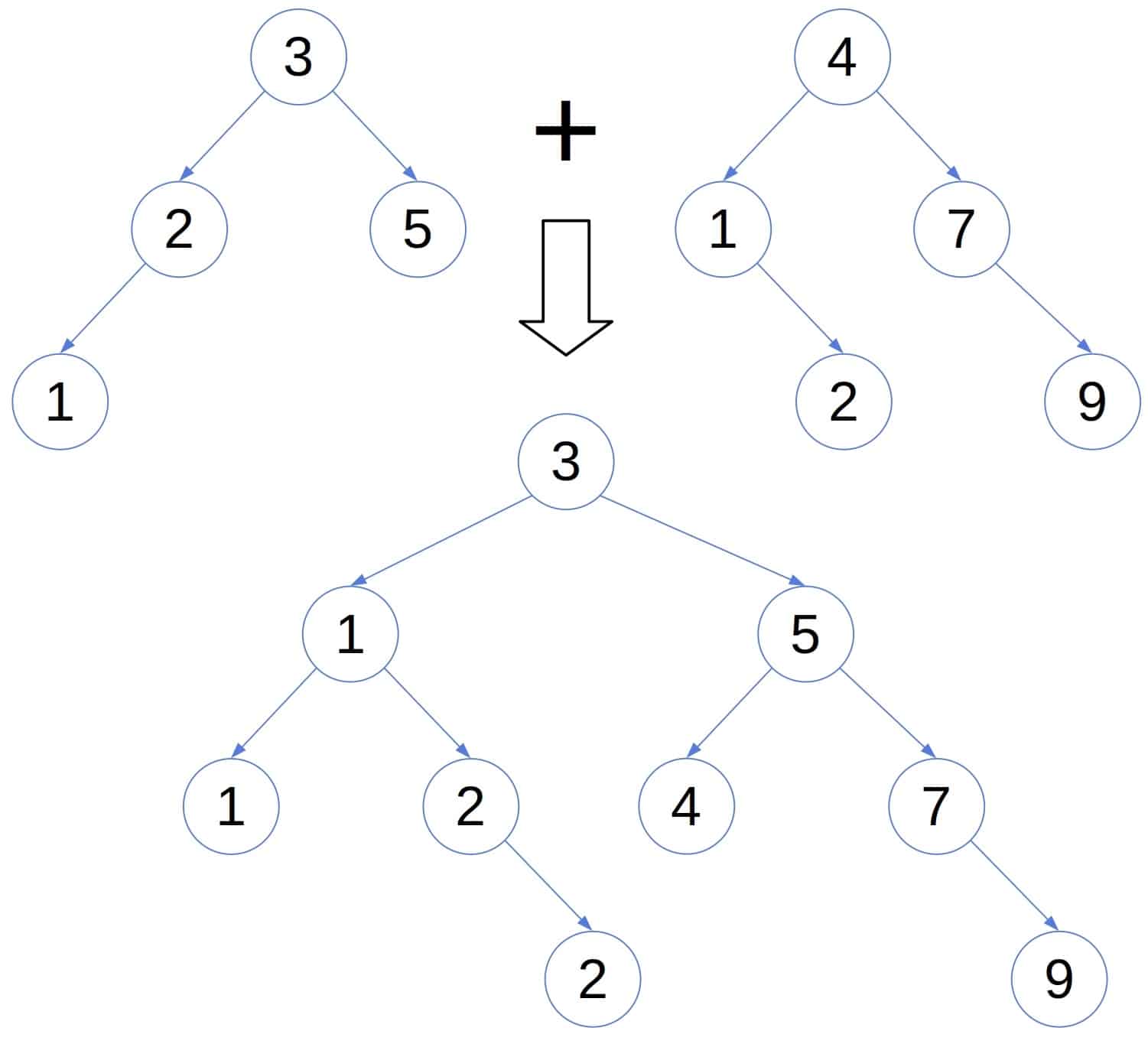
Merged BST has all the elements of BST1 and BST2 and maintains the characteristics of a binary search tree.

2. Merge, Sort, Reconstruct

In this algorithm, the main idea is to move the elements of both BSTs to an array, sort and form the merged BST.

This algorithm has the following 3 primary steps:

• step 1: Process the BSTs and store the elements in their respective arrays.
• step 2: Combine the arrays in a merged array and sort the elements in them. We can use any of the popular sorting methods such as bubble sort, insertion sort, etc.
• step 3: Copy the elements of the merged array to create merged BST by in-order traversing.

Since it increases with the size of the dataset, the complex it of step 1 is . The and are being the size of the BSTs that are merged.

The time complexity of step 2 depends on the type of the sorting algorithm used, it’ll be if it’s bubble sort and if it’s insertion sort.

We need to store all elements in the array, so the space complexity of the step is .

The algorithm can be described as follows:

algorithm mergeBSTsBySorting(BSTs):
    // INPUT
    //    BSTs = BSTs to be merged
    // OUTPUT
    //    A merged BST from the sorted array of all elements
    
    mergedArray <- an empty sequence 
    // Store BST data to arrays and merge
    for BST in BSTs:
        // Store the data of the current BST to an array
        bstArrays <- store BST data to array
        mergedArray <- merge bstArray into mergedArray

    // Sort the merged array of all BST elements
    sort(mergedArray)

    // Create Merged BST from the sorted array
    mergedBST <- create BST from sorted mergedArray
    return mergedBST

3. Traverse, Sort, Reconstruct

In this solution, we traverse the elements for both BSTs simultaneously and moved to the merged array.

This algorithm also has the following 4 primary steps:

• step 1: Process the BSTs and store the elements in their respective arrays.
• step 2: Create an array that has the size of , where and is the size of two of the BSTs that are being merged. This array will store elements of merged BSTs.
• step 3: Simultaneously traverse both arrays. While traversing, pick the smaller of the current elements and moved it to the merged array. Then progress with processing after removing the element that was picked earlier.
• step 4: Copy the elements of the merged array to create merged BST by in-order traversing

The time and space complexity of step 1 and step 2 is as the complexity increases with the size of the dataset.

The time complexity of step 3 is . The space complexity of the step is , where is the size of the dataset after arrays are merged.

The time and space complexity of step 4 is .

Let’s see how it looks like:

algorithm mergeBSTsByTraversing(BSTs):
    // INPUT
    //    BSTs = BSTs to be merged
    // OUTPUT
    //    A merged BST from traversing and merging elements of BSTs

    mergedArray <- an empty sequence that can accommodate all elements
    bstArrays <- an array of BST arrays for the input BSTs

    // Store BST data to arrays
    for index, BST in BSTs:
        bstArrays[index] <- store BST data to array
        mergedArray <- merge bstArray into mergedArray

    // Merge arrays by traversing nodes
    for node in mergedArray:
        // Assuming the function to traverse and compare nodes is implemented
        traverse and compare nodes of bstArrays[1] and bstArrays[2]
        move smaller element to merged

4. Conclusion

In this article, we looked at two possible solutions that can be used to merge binary search trees. Also, we identified the time and space complexity of each.