

Learn through the super-clean Baeldung Pro experience:
>> Membership and Baeldung Pro.
No ads, dark-mode and 6 months free of IntelliJ Idea Ultimate to start with.
Last updated: March 18, 2024
Learn through the super-clean Baeldung Pro experience:
>> Membership and Baeldung Pro.
No ads, dark-mode and 6 months free of IntelliJ Idea Ultimate to start with.
In this tutorial, we’ll introduce one of the algorithms of finding the lowest common ancestor in a directed acyclic graph. Also, we’ll talk about its time complexity.
Moreover, we’d see the difference in the algorithms of finding the lowest common ancestor in an undirected tree and in a directed acyclic graph. We assume having a basic knowledge of graphs and Big-O notation.
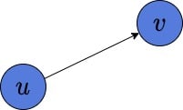
Let’s briefly remember the main definitions of a directed acyclic graph (DAG). A pair of vertices  is an edge. Furthermore, this edge has a direction from
  to
to  . Thus, it means is reachable from . However, is not reachable from :
The DAG is a graph, which contains no directed cycles. It means, that there is no vertex , such that we can find a path from and reach this vertex again.
The interesting thing is that we can build a DAG, but the corresponding undirected graph may or may not contain a cycle:
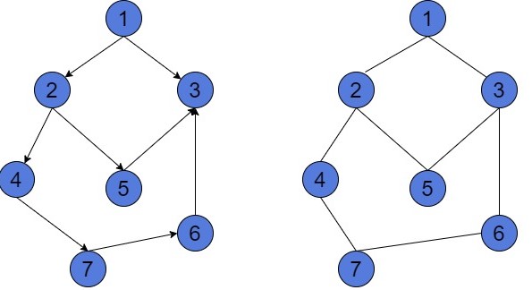
The graph to the left is DAG. It contains no directed cycles. To prove it, we may have a look at each contour and see this is not a cycle. For instance, the contour  is not a cycle, because the edge
  doesn’t exist in this graph. We have only edge
  . Similarly, we can prove that the other contours aren’t cycles.
However, if we’d remove the orientation of vertices, we’ll get the undirected graph to the right. This graph contains 3 cycles ,  and
and  . This happens because edges are undirected. And for every connected pair of vertices and we may assume that both edges and
  exist.
But, we can also build a DAG, such that the corresponding undirected graph will be acyclic:
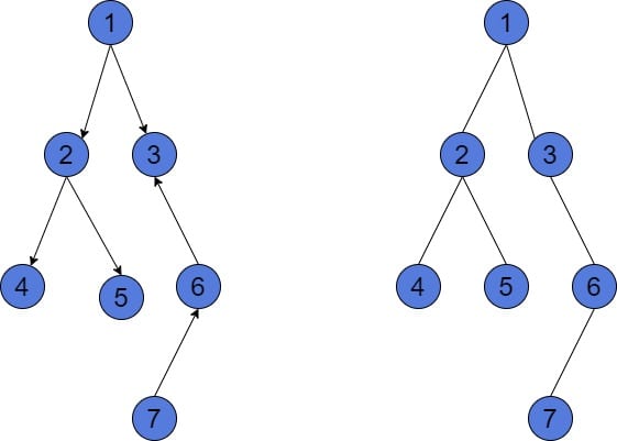
Both graphs in the picture are acyclic. The condition of an undirected graph of  vertices to be acyclic is to have at most
  edges. Assume we have a DAG of vertices and or fewer edges. So, we can be sure that the removal of its orientation will result in an acyclic graph as well.
However, the directed acyclic graph might have up to  edges.
Finding the lowest common ancestor (LCA) is a typical graph problem. It only makes sense to search for LCA in a rooted tree. However, the algorithms differ a bit from each other, depending on the type of the graph. Let’s shortly remember the problem definition.
The LCA between two nodes and in a graph is the deepest node  , such that it is an ancestor of both and . In case DAG is a special case of a graph, the might be 0, 1, or more LCAs between any two nodes. However, in an undirected tree, there will be exactly one LCA candidate.
Is important to notice, that for any nodes and , the  .
.
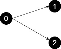
Each node of a graph has an in-degree and an out-degree. The in-degree is the number of incoming edges. The out-degree is the number of edges starting at this node (outcoming). The node is called a source if it has 0 in-degree. The node is called a leaf if it has 0 out-degree Let’s look at an example:
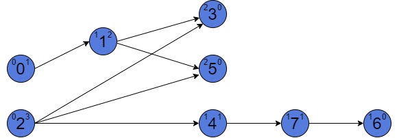
There are 3 numbers at each vertex of a graph in the picture. Those are the value of a vertex, and an in-degree and out-degree to the left and to the right of each value respectively. There are two sources in such a graph: 0 and 2. They both have zero in-degree. Also, there are three leaves: 3, 5, and 6. They have zero out-degree.
Is important to notice, the graph on the picture looks ordered. Actually, every directed acyclic graph has a topological order. Such an order of vertices might help us to better understand the algorithms.
A depth of a node in a directed acyclic graph,  , is the length of the longest path from the source node to . Also, there might be more than one source node. To compute the depth of each node, we can perform a Breadth-First Search (BFS). Here is an example of how depth can differ in similar DAGs:
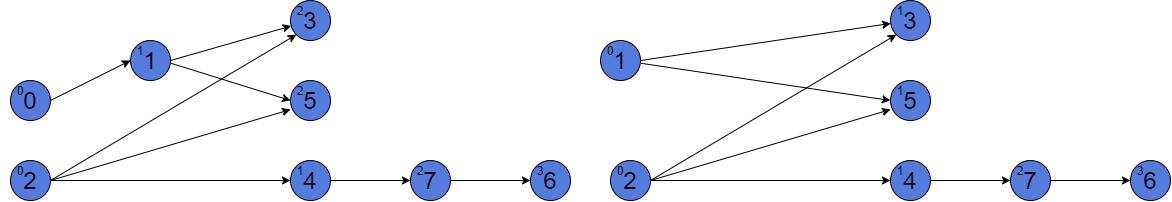
The number in the top left corner of each vertex is the depth of this node. The depth of the source is always 0. Let’s look at the graph to the left in the picture. The depth of node 5 is 2. It has two different paths from the source nodes 2 and 0. However, the depth of 5 is 2, because the depth is the longest path from any source node. But, if we remove vertex 0 from our graph (graph to the right in the picture), the depth of node 5 will be 1, because it has 2 paths from sources 1 and 2. Both paths are of length 1.
As we’ve mentioned, there might be more than one lowest common ancestor between two nodes. The numbers of LCAs in the directed acyclic graph might be between 0 and  , where
  is the number of vertices:
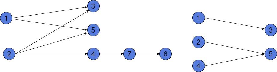
In the graph of 7 vertices, the  or
or  , because both 1 and 2 has equal depths. The
  and
and  .
.
If we want to find the LCA between a vertex and its ancestor, the LCA will be the ancestor. Thus, for instance, the  .
.
In the other graph, there exists no LCA between vertices 3 and 5. They have no parents in common.
We’ll introduce a simple algorithm, which is able to find all the lowest common ancestors between two given nodes of a graph.
Suppose we want to find the  in graph
  . Initially, all the vertices are colored white.
First, we do a Depth-First Search (DFS) on one of the target nodes. Let it be node . Also, we’ll keep track of the parent’s array (current path from a starting vertex). During the DFS, we color all the ancestors of in red each time we reach it.
Second, we should start the DFS on the other node . When we reach it, we recolor all red ancestors of in black.
Finally, we built a subgraph, induced by the black nodes. The nodes in a new graph with zero out-degrees are the answers.
Let’s visualize the algorithm steps:
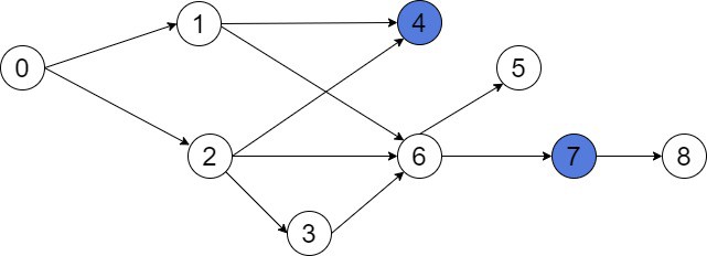
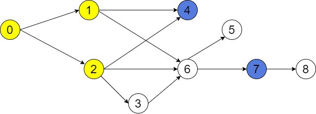
This is our initial graph. Suppose we want to find the LCA(4, 7). We start a DFS and color all parents of either 4 or 7 in red. For example, let’s choose vertex 7:
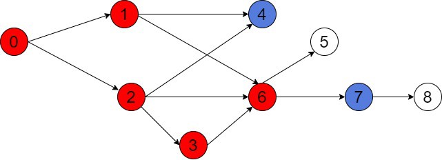
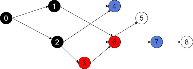
As we may see, node 7 has 5 parents. Then, we should color all parents of another node, which is 4, in black. For better understanding, we’ll first find all the ancestors of 4:
Vertex 4 has 3 parents. But, our aim is to color the intersection of red and yellow nodes in black. The intersection of  and
and  is . Thus, there are 3 black nodes:
The last step is to induce a subgraph on black nodes 0, 1, and 2. This will be a subgraph with 3 vertices and all common edges of 0, 1, and 2:
Now, we may see that two nodes 1 and 2 have zero out-degree. Therefore, they are the answer to our problem. The  or
or  .
.
We’ll assume we have the only source node in our graph.
The time complexity of such an algorithm is  , where is the number of vertices and
  is the number of edges in DAG . However,
  in DAG. During the algorithm, we sequentially do the DFS twice. After that, we built a subgraph, induced by the black nodes. Their amount might be at most , which is
  . The number of edges in a new subgraph might also be a
  . So, building an induced subgraph also takes . Finding the nodes with zero out-degree will take O(V) time.
So, the total time complexity of our algorithm is  .
.
However, if we’d have more than one source node, the time complexity will increase up to  . The additional multiplier represents that we should start DFS from all source vertices. Their amount might be up to . Then, we’ll have to find the intersection of all ancestors from all searches to find all the parents of a node.
In this article, we introduced one of the algorithms for finding the LCA between two vertices in a directed acyclic graph. Moreover, we noticed the difference in terminology and problem definition for the LCA problem for undirected trees and DAGs. Furthermore, we discussed our algorithm time complexity. Of course, there exist more efficient algorithms with precomputation techniques. However, they are not much faster than the proposed brute-force solution.