How to Perform Linear Discriminant Analysis? | Baeldung on Computer Science

1. Introduction

In this tutorial, we’ll delve into the intricacies of Linear Discriminant Analysis (LDA).

2. Dimensionality Reduction Techniques

Dimensionality reduction simplifies datasets by reducing dimensions and categorizing them into unsupervised and supervised approaches.

Unsupervised methods like principal component analysis (PCA) and independent component analysis (ICA) don’t require class labels, offering versatility. Supervised approaches like mixture discriminant analysis (MDA), neural networks (NN), and linear discriminant analysis (LDA) integrate class labels. Our focus is on LDA.

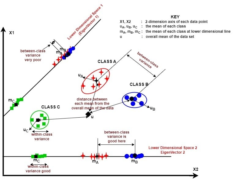
3. What Is Linear Discriminant Analysis (LDA)?

LDA is a powerful dimensionality reduction technique. It seeks to transform our data into a lower-dimensional space, enhancing class separability while minimizing within-class variance:

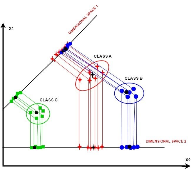
We observe three data clusters: class A, class B, and class C. Projecting along dimensional space 1 reduces within-class variance but loses between-class variance for classes A and B. Dimensional space 2 maintains both variances. Thus, we discard space 1 and use space 2 for LDA.

3.1. Steps to Performing LDA

In tackling dimensionality reduction with LDA, we divide the process into three main steps.

First, we maximize class separability by measuring the distance between their means (between-class variance)
Second, we minimize the closeness of each data point within a class to its mean (within-class variance)
Lastly, we use these parameters to construct an appropriate lower-dimensional space

The figure below illustrates these steps visually:

This newly constructed space simplifies our data and strengthens its power to distinguish between classes.

3.2. Approaches to LDA

Exploring LDA, we encounter class-dependent and class-independent approaches. In class-dependent LDA, each class gets its own lower-dimensional space. Conversely, class-independent LDA treats each class separately but shares one lower-dimensional space.

4. Mathematical Foundations of LDA

In this section, we discuss the mathematical process for performing LDA.

4.1. Calculating the Between-class Variance

To calculate the between-class variance $S_B$ , we follow the following steps:

We first calculate the separation distance $(m_i - m)$ as follows:

(1) $\begin{equation*}(m_i-m)^2 = (W^Tu_i - W^Tu)^2 = W^T(u_i - u)(u_i - u)^TW\end{equation*}$

where, $m_i$ represents the projection of the mean of the $i^{th}$ class which we calculate as follows:

$m_i = W^Tu_i$ .

$m$ is the projection of the total mean of classes which we calculate as follows:

$m = W^Tu$ ,

where $W$ represents the transformation matrix of LDA, $u_i$ represents the mean of the $i^{th}$ class and we calculate it as follows,

$u_i = \frac{1}{n_i}\sum_{x_i\in w_i}x_i$ .

$u$ is the total mean of all classes which we calculate as follows:

$u = \frac{1}{N}\sum_{i=1}^{N}x_i = \frac{1}{c}\sum_{i=1}^{c}u_i$ ,

where $c$ is the total number of classes.

The term $(u_i - u)(u_i - u)^T$ in equation 1 represents the between-class variance $S_{Bi}$ of the $i^{th}$ class.

We substitute $S_{Bi}$ into equation 1 as follows:

(2) $\begin{equation*}(m_i-m)^2 = W^TS_{Bi}W\end{equation*}$

We now obtain the total between-class variance $S_B$ as follows:

(3) $\begin{equation*}S_B = \sum_{i=1}^{c}n_{i}S_{Bi}\end{equation*}$

4.2. Calculating the Within-class Variance

To calculate the between-class variance $S_W$ , we take the following steps:

The within-class variance of the $i^{th}$ class $(S_{Wi})$ is the difference between the mean and the samples of that class.

We then search for a lower-dimensional space to minimize the difference between the projected mean $(m_i)$ and the projected samples of each class $(W^Tx_i)$ , which is the within-class variance.

We capture these steps with the equations as follows:

(4) $\begin{equation*}\sum_{x_i\in w_j}(W^Tx_i - m_i)^2 = \sum_{x_i\in w_j}W^T(x_i - u_i )(x_i - u_i )^TW = \sum_{x_i\in w_j}W^TS_{Wi}W\end{equation*}$

From equation 4, we calculate the within-class variance as follows;

$S_{Wi}$ = $d^T_i * d_i$ = $\sum_{k=1}^{n_i}(x_{ki} - u_i)(x_{ki} - u_i)^T$ ,

where $x_{ki}$ represents the $k^{th}$ sample in the $i^{th}$ class and $d_i$ is the centring data of the $i^{th}$ class, i.e.

$d_i$ = $w_i - u_i$ = $\{{x_k\}}_{k = 1}^{n_i} - u_i$ .

To calculate the total within-class variance of our data, we sum up the within-class variance of all classes present in our data as follows;

$S_W$ = $\sum_{i=1}^cS_{Wi}$ = $\sum_{x_i\in w_1}(x_i - u_1)(x_i - u_1)^T$ + $\sum_{x_i\in w_2}(x_i - u_2)(x_i - u_2)^T$ + … + $\sum_{x_i\in w_c}(x_i - u_c)(x_i - u_c)^T$ .

4.3. Constructing the Lower Dimensional Space: Fisher’s Criterion

To transform the higher dimensional features of our data into a lower dimensional space, we maximize the ratio of $S_B$ to $S_W$ to guarantee maximum class separability by using Fisher’s criterion $J(W)$ , which we write this way:

(5) $\begin{equation*}J(W) = \frac{W^TS_BW}{W^TS_WW}\end{equation*}$

To calculate the transformation matrix $W$ , we transform equation 5 into equation 6 as follows:

(6) $\begin{equation*}S_WW = \lambda S_BW\end{equation*}$

where $\lambda$ represents the eigenvalues of the transformation matrix $W$

Next, we transform equation 6 into equation 7 as follows:

(7) $\begin{equation*}W = S_W^{-1}S_B\end{equation*}$

we can then calculate the eigenvalues $(\lambda = {\lambda_1, \lambda_2,....,\lambda_M})$ and their corresponding eigenvectors $(V = v_1,v_2,....,v_M)$ of $W$ given in equation 7.

4.4. The Role of the Eigenvalues and Eigenvectors

In LDA, eigenvectors determine the direction of the space, while eigenvalues indicate their magnitude. We select the $k$ highest eigenvalue eigenvectors to form a lower dimensional space $V_k$ , neglecting others. This reduces our original data $X$ from dimension $M$ to $k$ . We write this new dimensional space $Y$ as:

(8) $\begin{equation*}Y = XV_k\end{equation*}$

5. Class-independent and Class-dependent LDA Approach

Here, we describe the slight difference between the class-independent and class-dependent LDA approaches and also provide the algorithms for both.

5.1. Class-independent LDA Approach

In the class-independent method, we use only one lower-dimensional space for all classes. Thus, we calculate the transformation matrix $W_i$ for all classes, and we project the samples of all classes on the selected eigenvectors.

Here is the algorithm for the class-independent LDA approach:

5.2. Class-dependent LDA Approach

In class-dependent LDA, we compute distinct lower-dimensional spaces for each class using $W_i = S_{W_i}^{-1}S_B$ . We find eigenvalues and eigenvectors for each $W_i$ separately, then project samples onto their respective eigenvectors.

We provide the algorithm for the class-dependent LDA approach as follows:

6. Computational Complexity of LDA

In this section, we provide the computational complexities of the two classes of LDA

6.1. Computational Complexity for Class-independent LDA

In analyzing the computational complexity of class-dependent LDA, we consider various steps. First, computing the mean of each class has complexity $O(DN + cD)$ . Second, calculating the total mean has complexity $O(ND + D)$ . Third, computing within-class scatter involves $O(ND + ND^2)$ . Fourth, calculating between-class scatter has complexity $O(cD + cD^2)$ . Fifth, finding eigenvalues and eigenvectors involves $O(D^3)$ . Sorting eigenvectors is $O(D \log D)$ . Selecting $k$ eigenvectors is $O(Dk)$ . Finally, projecting data onto eigenvectors is $O(DkN)$ . Overall, class-independent LDA has complexity $O(ND^2)$ for $N > D$ , otherwise $O(D^3)$ .

6.2. Computational Complexity for Class-dependent LDA

In analyzing computational complexity, both class-dependent and class-independent LDAs follow similar steps. However, class-dependent LDA repeats the process for each class, increasing complexity. Overall, class-dependent LDA complexity is $O(ND^3)$ for $N > D$ , or $O(cD^3)$ , surpassing class-independent LDA in complexity.

7. Numerical Example

In this section, we will present a numerical example explaining how to calculate the LDA space step by step and how LDA is used to discriminate two different classes of data using the class-independent and class-dependent approach.

The first class $w_1$ is a $5$ x $2$ matrix with the number of samples $n_1 = 5$ . The second class $w_2$ is a $6$ x $2$ matrix with $n_2 = 6$ . Each sample in both classes has two features (i.e., $D = 2$ ) as follows:

$w_1 = \begin{bmatrix} 2.3 & 1.2 \\ 0.8 & 2.0 \\ 5.1 & 1.5 \\ 6.2 & 4.4 \\ 3.8 & 0.9 \end{bmatrix}$ , and, $w_2 = \begin{bmatrix} 6.4 & 1.5 \\ 9.3 & 4.7 \\ 3.2 & 5.1 \\ 0.9 & 8.2 \\ 7.2 & 1.4 \\ 2.2 & 5.8 \end{bmatrix}$ .

First, we calculate the mean $u_j$ for each class, and then the total mean $u$ for both classes. The resulting answers are as follows;

$u_1 = \begin{bmatrix} 3.64 & 2.00 \end{bmatrix}$ , $u_2 = \begin{bmatrix} 4.87 & 4.45 \end{bmatrix}$ , and $u = \begin{bmatrix} 4.31 & 3.32 \end{bmatrix}$ .

Next, we calculate the between-class variance $S_{B_i}$ of each class, and the total between-class variance $S_B$ of the given data, as follows:

$S_{B_1} = n_1(u_1 - u)^T(u_1 - u)$ , so that,

$S_{B_1}= \begin{bmatrix} 2.24 & 4.47 \\ 4.47 & 8.93 \end{bmatrix}$

similarly,

$S_{B_2} = n_2(u_2 - u)^T(u_2 - u)$ , so that,

$S_{B_2}= \begin{bmatrix} 1.87 & 3.73 \\ 3.73 & 7.44 \end{bmatrix}$

$S_B$ becomes,

$S_B = S_{B_1} + S_{B_2} = \begin{bmatrix} 4.10 & 8.20 \\ 8.20 & 16.37 \end{bmatrix}$ .

Next, we calculate the within-class variance $S_W$ . To do this, we perform the mean-centering data process by subtracting the mean of each class from each sample in that class. We achieve this as follows: $d_i = w_i - u_i$ . Where $d_i$ is the mean-centering data of the class $w_i$ . The values of $d_1$ and $d_2$ becomes:

$d_1 = \begin{bmatrix} -1.34 & -0.80 \\ -2.84 & 0.00 \\ 1.46 & -0.50 \\ 2.56 & 2.40 \\ 0.16 & -1.10 \end{bmatrix}$ , and $d_2 = \begin{bmatrix} 1.53 & -2.95 \\ 4.43 & 0.25 \\ -1.67 & 0.65 \\ -3.97 & 3.75 \\ 2.33 & -3.05 \\ -2.67 & 1.35 \end{bmatrix}$ .

In the next two sub-sections, we’ll present how the two LDA approaches solve this numerical example.

7.1. Class-independent LDA Approach

In this approach, after the data centering process, we calculate the within-class variance $S_{W_i}$ as follows: $S_{W_i} = d_i^T * d_i$ . The values of $S_{W_i}$ is as follows:

$S_{W_1} = \begin{bmatrix} 18.57 & 6.31 \\ 6.31 & 7.86 \end{bmatrix}$ , and $S_{W_2} = \begin{bmatrix} 53.07 & -30.09 \\ -30.09 & 34.38 \end{bmatrix}$ .

$S_W$ becomes,

$S_W = S_{W_1} + S_{W_2}$ .

$S_W = \begin{bmatrix} 71.65 & -23.78 \\ -23.78 & 42.24 \end{bmatrix}$ .

Next, we calculate the transformation matrix $W$ as follows: $W = S_W^{-1}S_B$ . The values of $S_W^{-1}$ are $\begin{bmatrix} 0.02 & 0.01 \\ 0.01 & 0.03 \end{bmatrix}$ . The values of the transformation matrix become;

$W = \begin{bmatrix} 0.15 & 0.30 \\ 0.28 & 0.56 \end{bmatrix}$ .

We then calculate the eigenvalues $\lambda$ and eigenvectors $V$ from $W$ . Their values are as follows:

$\lambda = \begin{bmatrix} 0.00 & 0.00 \\ 0.00 & 0.71 \end{bmatrix}$ , and $V = \begin{bmatrix} -0.89 & -0.47 \\ 0.45 & -0.88 \end{bmatrix}$

Next, we project $w_1$ and $w_2$ onto the first column vector $V^{[1]}$ and the second column vector $V^{[2]}$ of the matrix $V$ to investigate which of the columns is more robust in discriminating the data.

Using $V^{[1]}$ , we project $w_1$ on the lower dimensional space as follows:

$y_1 = w_1V^{[1]}$ ,

$y_1 = \begin{bmatrix} 2.3 & 1.2 \\ 0.8 & 2.0 \\ 5.1 & 1.5 \\ 6.2 & 4.4 \\ 3.8 & 0.9 \end{bmatrix} \begin{bmatrix} -0.89 \\ 0.45 \end{bmatrix} = \begin{bmatrix} -1.52 \\ 0.18 \\ -3.89 \\ -3.57 \\ -3.00 \end{bmatrix}$

Using the same eigenvector $V^{[1]}$ , we project $w_2$ on the lower dimensional space as follows:

$y_2 = w_2V^{[1]}$ ,

$y_2 = \begin{bmatrix} 6.4 & 1.5 \\ 9.3 & 4.7 \\ 3.2 & 5.1 \\ 0.9 & 8.2 \\ 7.2 & 1.4 \\ 2.2 & 5.8 \end{bmatrix} \begin{bmatrix} -0.89 \\ 0.45 \end{bmatrix} = \begin{bmatrix} -5.05 \\ -6.21 \\ -0.58 \\ -2.87 \\ -5.81 \\ 0.63 \end{bmatrix}$ .

Next, we project $w_1$ and $w_2$ to eigenvector $V^{[2]}$ as follows:

$y_1 = w_1V^{[2]}$ ,

$y_1 = \begin{bmatrix} 2.3 & 1.2 \\ 0.8 & 2.0 \\ 5.1 & 1.5 \\ 6.2 & 4.4 \\ 3.8 & 0.9 \end{bmatrix} \begin{bmatrix} -0.47 \\ -0.88 \end{bmatrix} = \begin{bmatrix} -2.15 \\ -2.14 \\ -3.74 \\ -6.81 \\ -2.60 \end{bmatrix}$

and

$y_2 = w_2V^{[2]}$ ,

$y_2 = \begin{bmatrix} 6.4 & 1.5 \\ 9.3 & 4.7 \\ 3.2 & 5.1 \\ 0.9 & 8.2 \\ 7.2 & 1.4 \\ 2.2 & 5.8 \end{bmatrix}\begin{bmatrix} -0.47 \\ -0.88 \end{bmatrix} = \begin{bmatrix} -4.35 \\ -8.54 \\ -6.01 \\ -7.65 \\ -4.46 \\ -6.15 \end{bmatrix}$ .

From our results, we observe that $V^{[2]}$ is more robust in discriminating the classes $w_1$ and $w_2$ than $V^{[1]}$ . This is because $\lambda^{[2]}$ is larger than $\lambda^{[1]}$ . Hence, we choose $V^{[2]}$ to discriminate $w_1$ and $w_2$ instead of $V^{[1]}$ .

7.2. Class-dependent LDA Approach

In this approach, we aim to calculate a separate transformation matrix $W_i$ for each class $w_i$ . The within-class variance for each class is the same as we calculated it in the class-independent approach, we then calculate $W_i$ of each class as follows: $W_i = S_{W_i}^{-1}S_B$ . The values of $W_1$ and $W_2$ becomes:

$W_1 = S_{W_1}^{-1}S_B$

$W_1 = \begin{bmatrix} 18.57 & 6.31 \\ 6.31 & 7.86 \end{bmatrix}^{-1}\begin{bmatrix} 4.10 & 8.20 \\ 8.20 & 16.37 \end{bmatrix} = \begin{bmatrix} -0.18 & -0.37 \\ 1.19 & 2.38 \end{bmatrix}$ , and

$W_2 = S_{W_2}^{-1}S_B$

$W_2 = \begin{bmatrix} 53.07 & -30.09 \\ -30.09 & 34.38 \end{bmatrix}^{-1}\begin{bmatrix} 4.10 & 8.20 \\ 8.20 & 16.37 \end{bmatrix} = \begin{bmatrix} 0.42 & 0.84 \\ 0.61 & 1.21 \end{bmatrix}$ .

Next, we calculate the eigenvalues $\lambda_i$ and the corresponding eigenvectors $V_i$ of each transformation matrix $W_i$ .

The values of $\lambda_{w1}$ and $V_{w1}$ of $W_1$ for $w_1$ are as follows:

$\lambda_{w1} = \begin{bmatrix} 0.00 & 0.00 \\ 0.00 & 2.19 \end{bmatrix}$ , and the corresponding eigenvectors are; $V_{w1} = \begin{bmatrix} -0.90 & 0.15 \\ 0.45 & -0.99 \end{bmatrix}$

Similarly,the values of the eigenvalues $\lambda_{w2}$ and the corresponding eigenvectors $V_{w2}$ of $W_2$ for the second class data $w_2$ are as follows:

$\lambda_{w2} = \begin{bmatrix} 0.00 & 0.00 \\ 0.00 & 1.64 \end{bmatrix}$ , and the corresponding eigenvectors are; $V_{w2} = \begin{bmatrix} -0.90 & -0.57 \\ 0.45 & -0.82 \end{bmatrix}$ .

From the results above, we observe that $V_{w1}^{[2]}$ of $V_{w1}$ for $w_1$ has a bigger corresponding eigenvalue than $V_{w1}^{[1]}$ , this implies that $V_{w1}^{[2]}$ will discriminate $w_1$ better than the $V_{w1}^{[1]}$ , thus, we chose $V_{w1}^{[2]}$ as the lower dimensional space to project $w_1$ as follows;

$y_1 = w_1V_{w1}^{[2]}$

$y_1 = \begin{bmatrix} 2.3 & 1.2 \\ 0.8 & 2.0 \\ 5.1 & 1.5 \\ 6.2 & 4.4 \\ 3.8 & 0.9 \end{bmatrix}\begin{bmatrix} 0.15 \\ -0.99 \end{bmatrix} = \begin{bmatrix} -0.84 \\ -1.85 \\ -0.71 \\ -3.41 \\ -0.31 \end{bmatrix}$ .

For the second class $w_2$ , we also see that the second column eigenvector $V_{w2}^{[2]}$ of $V_{w2}$ has a higher eigenvalue than the first column eigenvector $V_{w2}^{[1]}$ , this also implies that $V_{w2}^{[2]}$ will discriminate better than the $V_{w2}^{[1]}$ . We obtain the projected data $y_2$ for $w_2$ as follows;

$y_2 = w_2V_{w2}^{[2]}$

$y_2 = \begin{bmatrix} 6.4 & 1.5 \\ 9.3 & 4.7 \\ 3.2 & 5.1 \\ 0.9 & 8.2 \\ 7.2 & 1.4 \\ 2.2 & 5.8 \end{bmatrix}\begin{bmatrix} -0.57 \\ -0.82 \end{bmatrix} = \begin{bmatrix} -4.90 \\ -9.16 \\ -6.01 \\ -7.25 \\ -5.26 \\ -6.02 \end{bmatrix}$ .

In the next sub-section, we present the visual illustration of the performance of LDA on the two classes of data $w_1$ and $w_2$ and then draw our conclusions.

7.3. Performance Analysis of Class-independent and Class-dependent LDA Approach

First, let us consider the class-independent LDA approach.

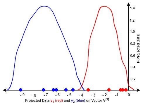
The next figures illustrate the probability density function (pdf) graphs of the projected data $y_1$ and $y_2$ on the two eigenvectors $V^{[1]}$ and $V^{[2]}$ of matrix $V$ :

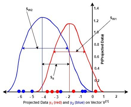
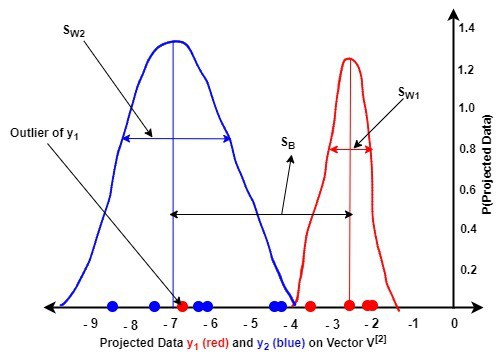
A comparison of the two figures reveals the following:

$V^{[2]}$ (second figure) showed a better discrimination of the data of each class than $V^{[1]}$ (first figure). This means that $V^{[2]}$ maximizes the between-class variance $S_B$ than $V^{[1]}$
$V^{[2]}$ minimized the within-class variance $S_{W_i}$ of the data of both classes than $V^{[1]}$
By using some techniques, we can easily handle the outlier of $y_1$ in the second figure

Let us investigate the class-dependent LDA approach:

We observe that by projecting $w_1$ onto $V^{[2]}$ of the first eigenvector and $w_2$ onto $V^{[2]}$ of the second eigenvector, we were able to discriminate the data efficiently. The corresponding eigenvectors achieved this by maximizing $S_B$ and minimizing $S_W$ of the data.

8. Conclusion

In our article, we explored linear discriminant analysis (LDA) through class-independent and class-dependent approaches. Our analysis revealed that while the class-dependent method is efficient, it demands more computational time than the class-independent approach. Consequently, the class-independent approach is commonly favoured as the standard method for LDA.

Full Archive

About Baeldung

Core Concepts

Operating Systems

Artificial Intelligence

Graph Theory

Latex