Best Data Structure for Dictionaries | Baeldung on Computer Science

1. Introduction

In this tutorial, we’ll give an overview of some ways to implement a dictionary.

2. What Is a Dictionary?

A dictionary is a collection of words associated with their meanings and possibly with references to other entries. Traditional paper dictionaries aren’t suitable for computational processing, so their digital counterparts have come to life and are nowadays used across various natural language processing (NLP) applications.

The data structure we use should support how we intend to use a dictionary. Most of the time, we’ll query the dictionary without adding new words or deleting new ones. However, we’ll also consider the case where changes are allowed.

Typically, a query will check for the presence of the query word in the dictionary. If it’s there, the query should return its definition. Otherwise, it should inform us that the word isn’t in the dictionary. Additionally, we may also be interested in range or prefix queries. We’ll discuss all those cases in this article.

3. Implementing a Dictionary

There are many ways to implement a dictionary, and their complexity and performance vary.

3.1. Sorted Arrays

In this approach, we maintain a dictionary as a sorted array of strings. Each string is a concatenation of a word and its definition, delimited by a special character. That way, by sorting the strings, we sort the words. The advantage of this method is that it’s simple to understand and implement. If we use binary search to find query words, a query will take $O(\log N)$ time in the worst case, where $N$ is the number of words in the dictionary.

A potential disadvantage is that if we have quite a lot of words to store, we may run out of main memory since arrays take up consecutive space. Since we need to keep the array sorted, this approach works best for static dictionaries. In such scenarios, we sort the array once and only allow searches afterward.

Further, although a single query is fast, querying a dictionary for $M$ words will have the time complexity of $O(M \log N)$ . So, in the long run, this may not be the best approach.

3.2. Hash Tables

Hash tables offer faster queries. Their lookup time is $O(1)$ in the average case, as long as we can fit them into our main memory. If we have a static dictionary and are interested in querying a word for its presence, perfect hashing would be the way to go. Its lookup time is constant even in the worst case.

Below is a small phonebook-like dictionary along with its metadata information (denoted as “D”), which uses a hash-table as its implementation:

With dynamic dictionaries, we want to be able to add new words, so we may need to resize our table. We can do that by making it two times larger every time it’s almost full. A drawback of dynamic dictionaries is the possibility of hash collisions. If we have too many words, some of them may end up getting hashed to the same key. So, we’ll need to introduce a mechanism to avoid collisions. That can make the complexity of queries linear in the worst case ( $O(N)$ ).

Finally, hash tables aren’t suitable for doing queries such as “find all words that share the same prefix or suffix”. That’s true for both static and dynamic dictionaries.

3.3. Tries

A trie is a data structure we often use when words can be broken down into lexemes (e.g., characters) and share prefixes with other words. A drawback is that tries are a bit memory inefficient in the standard implementation, but we can use compressed variants like Radix Trees, Succinct Trees, Directed Acyclic Word Graph (DAWG), and others.

As compared to the hash table for storing a fixed set of words, tries take less storage space but execute single-word queries slower. Another advantage is they don’t need any hash functions. Also, they naturally support prefix queries.

Here’s an example of a static dictionary we implemented as a trie:

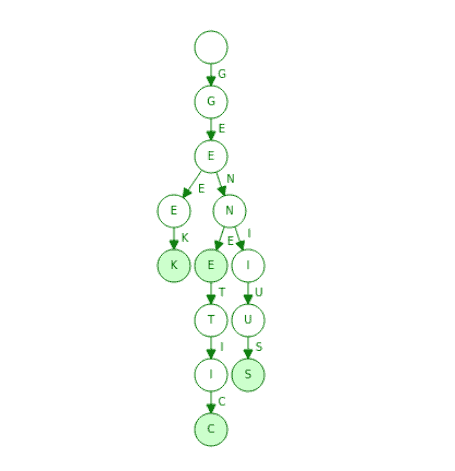
As we see, the trie stores the dictionary with the words “geek”, “gene”, “genius” and “genetic”. The shaded green nodes indicate the ends of the words, which may contain pointers to corresponding definitions.

A static dictionary can be easily built by inserting the words into our trie. The complexity of compiling a dictionary is $O(W*L)$ , where $W$ is the number of words and $L$ is the average word length. Once built, the structure is ready for querying for prefixes, suffixes (via suffix trees), or complete words. The complexity for a query for the word with $M$ characters is $O(M)$ . In contrast, the worst-case lookup for a hash table could be $O(N)$ where $N$ is the total words in the table.

In case we need a dynamic dictionary, we can easily grow our trie. Tries support insertion and deletion operations out of the box with the time complexity of $O(L)$ . Once we complete the updates, the structure is queryable again.

3.4. Bloom Filters

A Bloom Filter (BF) is a space-efficient probabilistic data structure. We use it to efficiently check if a word exists in our dictionary. The false negatives are impossible: if the filter can’t find a word, it isn’t there. The penalty we pay for efficiency is the possibility of a false positive. In simpler words, a query returns either “possibly in the dictionary” or “definitely not in the dictionary”. Other famous variants of BFs include blocked Bloom filters, Cuckoo filters, and others.

A bloom filter, if leveraged as a dictionary, doesn’t store the words in it. Instead, it keeps track of their memberships. So, a bloom filter serves as a lookup cache. This is the same idea as a hashmap, but it’s more space efficient.

Here’s what a Bloom Filter which uses 3 hash functions looks like:

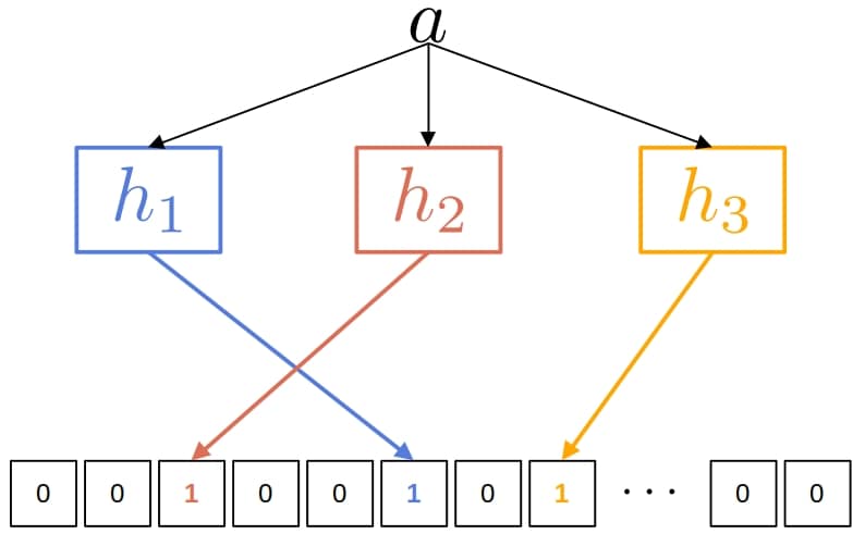
BF typically involves leveraging an array of $m$ bits and $k$ independent hash functions. In the above image, we are trying to add the word $a$ into our filter. The bits at the positions $h1(a) \bmod m$ , $h2(a) \bmod m$ , and $h3(a) \bmod m$ are all set to $1$ .

At the time of querying for $a$ , there should be no bits with value $0$ at the indexes marked by $h1(a) \bmod m$ , $h2(a) \bmod m$ , and $h3(a) \bmod m$ . If any is zero, that means the query word is certainly not in our BF. If all the bits are one, then the query word may or may not be in our dictionary.

BFs can be used as static or dynamic dictionaries as they support easy insertion, but deletion isn’t supported directly. There’s no limit on how many words we can store in BF but inserting a lot of words will drive the FP rate to be 100%, making the filter useless. It’s good to know the estimated number of words we want to store in BFs upfront.

When paired with a hash map, BFs can easily retrieve the definition of the query word if it’s there. It might seem counterintuitive but BFs can serve as an efficient lookup cache in front of the underlying hash map. With BFs resolving the incoming query words with a small amount of memory overhead, we can filter out which words aren’t there in the hashmap. As a result, we query our hash map only when we are confident that the definition possibly exists.

4. Conclusion

In this article, we talked about implementing a digital dictionary of a natural language.

Which way to go is very task-dependent. For a given set of words, if we are concerned with “is this word in it?”, a standard hash table is a very reasonable approach. We can use Bloom Filters if we are comfortable with some false-positive errors on key lookup. On the other hand, tries can check for a prefix or suffix, not just a complete word.

Full Archive

About Baeldung

Core Concepts

Operating Systems

Artificial Intelligence

Graph Theory

Latex