

Learn through the super-clean Baeldung Pro experience:
>> Membership and Baeldung Pro.
No ads, dark-mode and 6 months free of IntelliJ Idea Ultimate to start with.
Learn through the super-clean Baeldung Pro experience:
>> Membership and Baeldung Pro.
No ads, dark-mode and 6 months free of IntelliJ Idea Ultimate to start with.
In this tutorial, we’ll learn about  -armed bandits and their relation to reinforcement learning. We’ll then inspect the exploration and exploitation terms and understand the need to balance them by investigating the exploration vs. exploitation tradeoff.
Finally, we’ll investigate different strategies to get the maximum reward from a -armed bandit setting and how we can compare different algorithms using regret.
The one-armed bandit is a slang term for slot machines. Although the chances are slim, we know that spinning the one-armed bandit has a probability of winning. This means, given enough trials, we’ll win at some point. We just don’t know the probability distribution and can’t discover it with a limited number of trials.
Now imagine we’re in a casino, sitting in front of 10 different slot machines. Each one of the slot machines has a probability of winning. If we have some coins to play, which one do we choose? Do we spend all our chances on a single machine, or do we play on a combination of different machines?
Finding the optimal playing strategy to win the highest possible reward isn’t a trivial task. We’ll learn about strategies for solving the  -armed bandit in the following sections.
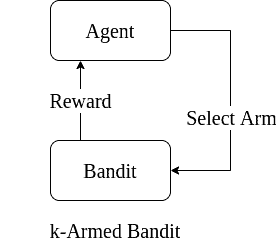
In reinforcement learning, an agent is interacting with the environment. It’s trying to find out the outcomes of available actions. Its ultimate goal is to maximize the reward at the end.
The -armed bandit problem is a simplified reinforcement learning setting. There is only one state; we (the agent) sit in front of k slot machines. There are actions: pulling one of the distinct arms. The reward values of the actions are immediately available after taking an action:
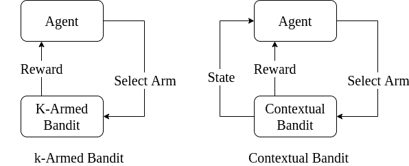
 -armed bandit is a simple and powerful representation. Yet, it can’t model complex problems ignoring the consequences of previously taken actions.
To better model the real-life problems, we introduce the “context”. The agent selects an action, given the context. In other words, the agent has a state, and taking actions makes the agent transition between states and results in a reward. Simply put, context is the result of previously taken actions:
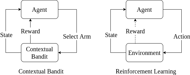
Still, the reward is immediate after choosing an action in the contextual bandit model, unlike real-world problems. Sometimes we get a reward after some time or after taking a series of actions. For example, even in simple games like tic-tac-toe, we receive the reward after making a series of moves when the game ends. Hence, contextual bandits are too simplified to model some problems:
In a -armed bandit setting, the agent initially has none or limited knowledge about the environment. As a result, it discovers the environment by trial-and-error.
Let’s consider the -armed bandit setting. Here, we know that each of the slot machines gives an immediate reward, based on a probability distribution. The reward will be a real number, negative or positive. The figure below illustrates an example setting with = 10:
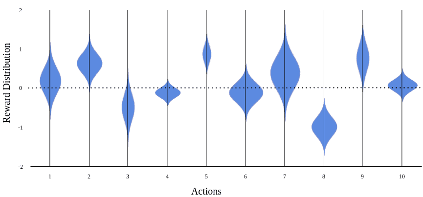
Although the reward distribution of each slot machine is determined in this setting, we don’t know about them. So, we’ll try to discover by trial-and-error. Choosing an arbitrary action when the outcome is unknown is called exploration.
Say we choose random actions in this unknown setting (explore). As a result, after some time, we have an initial idea about each slot machine’s reward. With a small number of trials, we can’t be confident about the expected values. Still, we know something about the environment at this point.
In our example setting, the blue dots mark what the agent believes the expected reward from a slot machine is. The light blue marks show the real distribution, which is still unknown to the agent at this point. For some machines, the agent’s expectation is close to average, while for some, it’s around the extremes after a limited exploration:
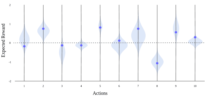
Taking actions according to the expectations and using prior knowledge to get immediate rewards is called exploitation. In our example, the agent would exploit by choosing the 5th machine, as it believes it’ll result in a positive reward, and that would be a good choice. However, the agent would try the 6th machine in a similar belief, which wouldn’t meet its expectations.
Depending on the problem size, after enough trials, the agent has a better estimation of the slot machines’ expected reward values. As a result of exploration, now the agent’s expectations highly match the actual rewards:
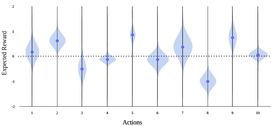
In a realistic reinforcement learning problem with many states and actions, it takes an infinite number of trials to actually learn the environment and accurately predict the expected rewards. Even at times, the environment might be changing (non-stationary). So, sticking to what we’ve already learned isn’t a good idea. It’s risky and even dangerous in some cases, as the agent can get stuck in a sub-optimal choice.
On the other hand, constantly exploring the environment means only taking random actions. Not exploiting a good reward opportunity is simply against the overall goal of getting the maximum overall reward.
In such a setting containing incomplete information, we need to have a balance. The best long-term strategy may involve taking short-term risks. Exploration can lead to higher reward in the long run while sacrificing short term rewards. Conversely, exploiting ensures an immediate reward in the short-term, with uncertainty in the long run. The dilemma of choosing what the agent already knows vs. gaining additional knowledge is called the exploration vs. exploitation tradeoff.
The -armed bandit environment contains uncertainties. The exploration vs. exploitation trade-off arises due to incomplete information. If we were to know everything about the environment, then we could find an optimal solution. However, real-world problems involve many unknowns.
One way to evaluate -armed bandit strategies is to measure the expected regret. As the name suggests, lower regret values are better.
We measure the expected regret at each action. When an action is taken, we have an approximation for the expected reward of the best possible action. Besides, we instantly get the reward for the taken action. The difference between the expected best reward and the actual reward gives the expected regret. It denotes what we’ve lost by exploring instead of taking the best action.
We can compare different strategies on a given problem by cumulatively adding the regret values and comparing the results.
Now let’s explore some strategies for approximating a good solution for the -armed bandit problem.
The explore-first (or epsilon-first,  -first) strategy consists of two phases: exploration and exploitation.
As the name suggests, in the exploration phase, the agent tries all options several times. Then, it selects the best action based on those trials. Finally, in the exploitation phase, it just takes the action with the best outcome.
The exploitation phase of this algorithm works perfectly in terms of minimizing regret. However, the inefficiency lies in the exploration phase. The overall performance isn’t satisfactory for most applications.
In the epsilon-greedy ( -greedy) approach, instead of having a pure exploration phase, we spread the exploration over time.
Initially, we select a small epsilon value (usually, we choose  ). Then, with a probability of epsilon, even if we’re confident with the expected outcome, we choose a random action. On the remaining times (1 – epsilon), we simply act greedy and exploit the best action. We apply this simple algorithm for the whole period.
The epsilon-greedy algorithm is easy to understand and implement. It’s one of the basic reinforcement learning enhancements with Q-learning.
A downside of the epsilon-greedy strategy is that the exploration phase is uniformly distributed over time. We can improve on this by exploring more in the beginning, when we have limited knowledge about the environment. Then, as we learn, we can make more educated decisions and explore less.
The idea is pretty simple to implement. We introduce a decay factor (usually around 0.95). After each action, we update epsilon to be epsilon*decay. So, the epsilon value gradually decreases over time. This results in lowering the regret compared to the epsilon-greedy algorithm.
The softmax approach enables us to select an action with a probability depending on its expected value. Remember that the epsilon-greedy approach selects a uniform random action while exploring. So, the second-best option and the worst option have the same probability of being selected.
In softmax exploration, the agent still selects the best action most of the time. However, other actions are ranked and selected accordingly. As a result, it’ll behave better than the epsilon-greedy. Still, the regret is not bounded.
Pursuit methods maintain both action-value estimates and action preferences for the current state. Their preference continually “pursuit” the best (greedy) action according to the current estimates.
The action preference probabilities are updated before action selection. The probability of choosing the best actions is increased, and others’ probabilities are decreased.
Upper confidence bounds (UCB) is a family of algorithms trying to balance exploration and exploitation.
At first, we ensure that each action is taken at least once for every state. Then, when we face a selection again, we select the action maximizing the upper confidence bound.
UCB improves quickly and converges more rapidly than the other methods. The algorithm selects the optimal action as the number of trials goes to infinity.
Its overall regret grows logarithmic, and it’s bounded. Hence, theoretically, it’ll be the best performing strategy in the long run.
The algorithms we’ve discussed so far update the expected reward per action using the mean of previous trials. Thompson sampling algorithm adopts a different approach.
It assumes that each action offers a reward based on a beta probability distribution and tries the estimate the distribution within a confidence interval. The priority distribution of the action is updated after taking an action. Then the algorithm chooses the action that maximizes the expected reward.
In this sense, the Thompson sampling algorithm adopts a Bayesian Inference approach, where the setting is updated as more evidence becomes available.
The figure below compares the worst-case bounds for some of the algorithms:
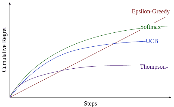
In most settings, epsilon-greedy is hard to beat. UCB and Thompson Sampling methods use exploration more effectively. Thompson sampling will be more stable, given enough trials. But, UCB is more tolerant of noisy data and converges more rapidly.
Depending on the problem at hand, a strategy can behave much better than the theoretical worst cases. Plotting the actual regret graphs of different algorithms might give different insights.
In this tutorial, we explored the -armed bandit setting and its relation to reinforcement learning. Then we learned about exploration and exploitation. Finally, we investigated various approximation techniques to solve the -armed bandit problem and how to evaluate and compare them using regret.