An Efficient Compression Algorithm for Short Text Strings

1. Overview

Data compression is a technique used to reduce the amount of data needed to represent a piece of information. It is essential in many areas, such as data storage, transmission, and archiving.

In this tutorial, we’ll focus on an efficient compression algorithm for short text strings.

We’ll explore the Burrows-Wheeler Transform (BWT) algorithm and how to combine it with the Run-Length Encoding (RLE) compressing algorithm to achieve a better compression ratio.

2. RLE Compression Algorithm

There are two main types of compression: lossless and lossy. Lossless compression guarantees that the data can be recovered exactly as it was before compression, while lossy compression may result in some loss of information. Let’s dive deeper into the lossless compression techniques.

2.1. What Is RLE Compression Technique?

Run-Length Encoding (RLE) is a way to compress data without losing any information (lossless compression). It replaces consecutive repeating characters with a single character and a number representing the number of times it appears. For example, the string can be compressed to .

Here’s how it works:

• First, we need to scan through the input data while looking for consecutive repeating characters
• Then, when we find a consecutive repeating character, we’ll replace it with the character followed by the number of times it appears
• Finally, the compressed output is the modified input data with repeating characters replaced

2.2. RLE Compression Algorithm

Let’s now look at the implementation of the RLE compression algorithm. Here’s a pseudocode for implementing the BWT algorithm:

algorithm RLE(s):
    // INPUT
    //    s = string
    // OUTPUT
    //    compressed_string = the string after applying RLE compression

    compressed_string <- an empty string // store the compressed output
    i <- 0

    while i < length(s):
        // count occurrences of character at index i
        count <- 1

        while i + 1 < length(s) and s[i] = s[i + 1]:
            count <- count + 1
            i <- i + 1
        // append current character and its count to the result
        compressed_string <- compressed_string + string(count) + s[i]
        
        i <- i + 1

    return compressed_string

The RLE method compresses repetitive sequences of characters in the input into shorter, more concise representations. As a result, the output is a compressed string containing the number of times a character appears in a row as well as the character itself.

The time complexity of the above solution is , where is the length of the input string and doesn’t require any extra space.

2.3. Example

Let’s say we have the following string: :

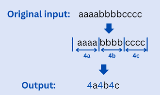
Using RLE, we would compress to . As we can see, the compressed output is smaller in size than the original one, but when we decode it, it will give us the original string back. This is the basic concept of RLE, which help in data compression.

By compressing the repeating sequences in the input into shorter representations, this technique reduces the total size of the data. However, the RLE compression technique is not necessarily the most efficient form of data compression. Its performance varies depending on the data being compressed. This is when the BWT algorithm comes into play.

3. Burrows-Wheeler Transform

To improve the compression of short text strings, we’ll now explore the Burrows-Wheeler Transform (BWT) algorithm, a specific technique that is known for its efficiency in this area.

3.1. What Is the BWT?

We are now ready to learn about the BWT. It’s a powerful data transformation method that is used in a lossless data compression algorithm. This makes it a great option for compressing sensitive data or important files.

One of the key features of BWT is its ability to group together similar characters in a string, which is a key factor in achieving efficient compression. Here’s how it works:

• First, we take the original string and create a matrix of all possible rotations of it
• Then, we sort these rows of the matrix in a lexicographic order
• Finally, we take the last column of the sorted rotations, which is the BWT of the original string. It’s simple yet powerful

3.2. BWT Transformation

Let’s now take a look at the implementation of the BWT transformation. Here’s an algorithm for implementing the BWT transformation:

algorithm BWT(s):
    // INPUT
    //    s = string
    // OUTPUT
    //    bwt = the Burrows-Wheeler Transform of the input string

    rotations <- create_rotations(s)
    sorted_rotations <- sort(rotations)
    bwt <- last_column(sorted_rotations)

    return bwt

The overall algorithm for the BWT transformation is quite simple. First, the algorithm takes a string as input. Next, we create all possible rotations of the string. Then, we sort them lexicographically. Finally, we get the last column of the sorted rotations, which is the BWT of the original string.

The BWT algorithm can be broken down into just three simple steps. Let’s take a look at the three functions that are used in the BWT approach:

• create_rotations(s): this function takes a string as input and creates a list of all possible rotations (using cyclic rotation) of the string. For example, if the input string is “banana$”, the function will return a list containing [“banana$“, “$banana“, “a$banan“, “na$bana“, “ana$ban“, “nana$ba“, “anana$b“]
• sort(rotations): this function takes a list of rotations as input and sorts them lexicographically (where the “$” sign is viewed as the first letter lexicographically) [“$banana“, “a$banan“, “ana$ban“, “anana$b“, “banana$“, “na$bana“, “nana$ba“]
• last_column(sorted_rotations): this function takes a list of sorted rotations as input and returns the last column of the rotations. This last column is the BWT of the original string BWT(banana$) = annb$aa

3.3. Inverse BWT

After the transformation of a string, we need to recover the original data. Here are the steps for implementing the inverse BWT (IBWT):

1. First, let’s initialize a table T with one row for each character in BWT(S) and one column for each character in BWT(S)
2. Second, we fill the first column of T with the characters of BWT(S)
3. Then, we sort the rows of T lexicographically
4. For to , where is the length of BWT(S):
   1. For each row of T, we append the character of BWT(S) to the beginning of the row
   2. Then, we sort the rows of T lexicographically
5. Let’s now find the row in T that ends with the end-of-file ($) character. This row corresponds to the original input string S
6. Return the string in that row, without the end-of-file character ($)

4. BWT Example

Let’s look at how to transform a string with the BWT transformation method and how to recover the original string after transformation.

4.1. BWT Transformation

Let’s say our string is “DOGWOOD“. To make things easier, we’ll add a special character, “$”, to the end of the string. This end character doesn’t appear anywhere in the original string. Here’s an example of applying the BWT approach on the string “DOGWOOD$” to obtain “DO$OODWG” as an output:

4.2. Recovering the String

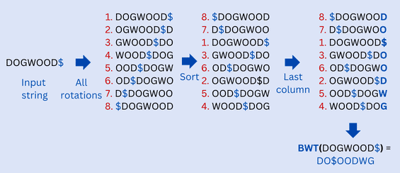
We have “DO$OODWG” as the transformed string of the BWT method. Let’s apply the IBWT approach to recover the original string “DOGWOOD“:

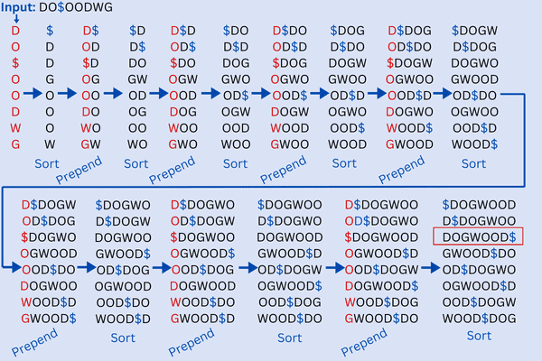
As we can see, we repeat the process of prepending a column of characters of the string “DO$OODWG” and sorting the rows of the obtained matrix until the number of columns of the matrix reaches the length of the input. This means the number of columns is equal to the number of rows. Then, we search for the row that has the end-of-file ($) character. This row corresponds to the original input string “DOGWOOD$”.

5. BWT + RLE Compression Method

Let’s now combine the RLE with the BWT to enhance the data compression.

5.1. BWT + RLE Algorithm

Here’s a pseudocode for implementing BWT followed by RLE:

algorithm BWTRLE(s):
    // INPUT
    //    s = string
    // OUTPUT
    //    compressed_string

    bwt <- BWT(s)
    compressed_string <- RLE_compress(bwt)

    return compressed_string

The RLE_compress(bwt) function used in the implementation takes the BWT-transformed string as input and applies the RLE compression algorithm to return the compressed string.

5.2. Example of BWT + RLE

Let’s use an example to make everything clear. Let’s say our string is “ABCABCABC“. As we can see, if we compress it using the RLE method we obtain “1A1B1C1A1B1C1A1B1C” as the compression output. This output has doubled the size of the original data. This is definitely not what we want as a result of using the compression method.

Let’s now apply the BWT approach to the string before the compression. Here’s an example of applying the BWT approach on the string “ABCABCABC“:

Transformation
Input	All Rotations	Sort the Order	Last Column	Output
ABCABCABC	ABCABCABC	3CA	ABCABCABC
	CABCABCABC		ABCABCABC	ABCABCABC
	BCABCABCABCA		BCABCAB	BCABCABCA
	ABCA		BCABCABCABCABCA	CABCABCAB
	CABCAB		CABCABCABCABC	CABCABCAB

Our final result is “CCC$AAABBB”, which is the BWT of the original string. Let’s now take a look at the chunks of repeated characters, like the ‘s. This is where compression comes in. The output “CCC$AAABBB” can be stored as “3C$3A3B” using the RLE to compress it.

6. Advantages and Disadvantages of BWT

Same as any approach, BWT has its benefits and drawbacks. Let’s then take a look at the benefits and drawbacks of the BWT in data compressing:

7. Conclusion

In this tutorial, we have discussed the RLE algorithm and how it can be used to compress short text strings efficiently.

We have also explored how combining BWT with the RLE compression technique can result in even better compression ratios. We have provided pseudocode examples to give a better understanding of the implementation of the algorithm.