

Learn through the super-clean Baeldung Pro experience:
>> Membership and Baeldung Pro.
No ads, dark-mode and 6 months free of IntelliJ Idea Ultimate to start with.
Last updated: February 28, 2025
Learn through the super-clean Baeldung Pro experience:
>> Membership and Baeldung Pro.
No ads, dark-mode and 6 months free of IntelliJ Idea Ultimate to start with.
We use loss (cost) functions to train and measure the performance of machine learning models, including neural networks.
In other words, the cost and loss estimate how well we train our networks. As a result, it’s crucial to choose a loss function appropriate for the task at hand, and there are many of them.
In this tutorial, we go over two widely used losses, hinge loss and logistic loss, and explore the differences between them.
The use of hinge loss is very common in binary classification problems where we want to separate a group of data points from those from another group. It also leads to a powerful machine learning algorithm called Support Vector Machines (SVMs) Let’s have a look at the mathematical definition of this function.
Let’s assume that  is the label of a data point in the training set. In addition, let’s say that
  is the model’s prediction for that sample.
Then, we define the hinge loss as follows:
![\[ L (x, y, w) = \text{max}(1 - m, 0)\]](/wp-content/ql-cache/quicklatex.com-9c2fe16d8bd9ff90db7cf70a73a1582a_l3.svg "Rendered by QuickLaTeX.com")
where  .
.
When a sample’s prediction  and has the same sign as the true label
  , then
  and the loss is zero. This means that for the correctly classified samples that are far from the margins, the model doesn’t incur any losses.
Between the margins ( ), however, even if a sample’s prediction is correct, there’s still a small loss. This is to penalize the model for making less certain predictions.
Below, we visualize the hinge loss:
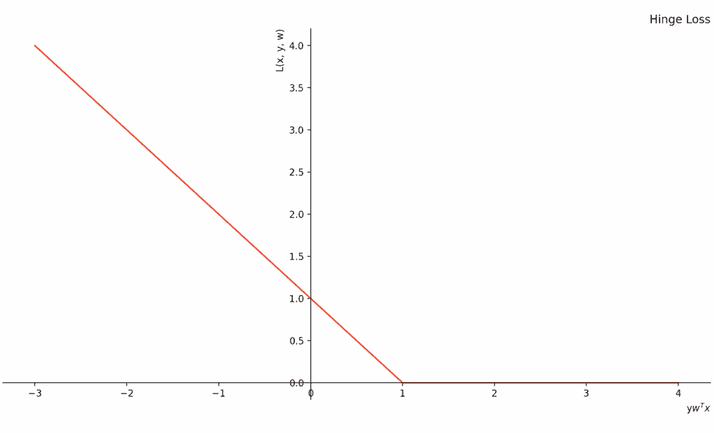
One of the main characteristics of hinge loss is that it’s a convex function. This makes it different from other losses such as the 0-1 loss. With convexity comes the existence of a global optimum. That’s a desirable property since we know how to find it with convex optimization algorithms such as gradient descent.
Another feature of hinge loss is that it leads to sparse models. The reason is that when solving the corresponding optimization problem, most of the training samples don’t play a role in the resulting discriminator. The ones that contribute to the margin between classes are called support vectors in the SVM model.
A negative property of the hinge loss is that it isn’t differentiable at one. This is problematic because we can’t use optimization algorithms such as LBFGS that work on differentiable functions. Consequently, this makes the function less suitable for large-scale problems which require an algorithm that uses linear memory usage (e.g. LBFGS).
Logistic loss (also known as the cross-entropy loss and log loss) is another loss function that we can use for classification. Minimizing this loss is equivalent to Maximum Likelihood Estimation.
Considering the same setting as the one for the hinge loss above, the logistic loss is defined as follows:
![\[ L (x, y, w) = \ln(1 + e^{-m})\]](/wp-content/ql-cache/quicklatex.com-4ba98313d788bfde9706ad1f6b7d5691_l3.svg "Rendered by QuickLaTeX.com")
where  .
.
Below, we can see what logistic loss looks like:
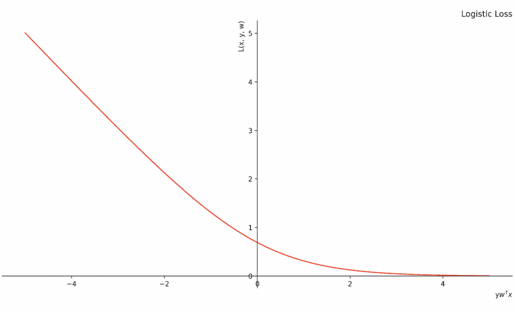
We see it’s a smooth function.
In contrast to the hinge loss which is non-smooth (non-differentiable), the logistic loss is differentiable at all points. That makes the function scalable to large-scale problems where there are many variables.
Logistic loss models the conditional probability  allowing it to naturally perform calibration as well. Subsequently, this makes the resulting model’s probability estimates more precise.
On the flip side, the logistic loss doesn’t necessarily maximize the margin between classes since it takes into account all the samples in both classes.
Based on the definitions and properties of the two loss functions, we can draw several conclusions about their differences.
Firstly, while both functions benefit from their convexity property, the logistic loss is smooth whereas the hinge loss isn’t. This makes the former more suitable for large-scale problems.
Secondly, while hinge loss produces a hyperplane separating the classes, it doesn’t give us any information on how certain it is about the membership of the samples. Logistic loss, on the other hand, models the conditional probability and thus, the probability estimates are its byproducts.
In terms of accuracy, the “No Free Lunch Theorem” asserts that we can’t say that one is better than the other in all possible settings. Generally speaking, however, since the logistic loss function considers all the data points, it could be more prone to outliers leading to lower accuracy than the hinge loss. This doesn’t happen to hinge loss because, as mentioned above, it ignores most samples and considers only the points nearest to the separating hyperplane.
Considering the size of the margin produced by the two losses, the hinge loss takes into account only the training samples around the boundary and maximizes the boundary’s distance from them. In contrast, the logistic loss might not produce maximum margins. The reason is that all the samples affect it. Any data point might shift the dividing hyperplane towards either class.
One advantage of hinge loss over logistic loss is its simplicity. A simple function means that there’s less computing. This is important when calculating the gradients and updating the weights. When the loss value falls on the right side of the hinge loss with gradient zero, there’ll be no changes in the weights. This is in contrast with the logistic loss where the gradient is never zero.
Finally, another reason that causes the hinge loss to require less computation is its sparsity which is the result of considering only the supporting samples.
To summarize, here are the features of the hinge loss versus the logistic loss:
| Feature | Hinge Loss | Logistic Loss |
|---|---|---|
| convexity | ✓ | ✓ |
| differentiability and smoothness | ✗ | ✓ |
| sparsity | ✓ | ✗ |
| cheaper computation | ✓ | ✗ |
| possibility of better accuracy | ✓ | ✗ |
| calibration | ✗ | ✓ |
In this article, we described the hinge and the logistic loss functions and explored their differences such as differentiability and simplicity. These properties determine their applicability to various problems.
The hinge loss isn’t differentiable everywhere but is convex and simple to compute and optimize. The logistic loss is differentiable everywhere but doesn’t necessarily produce the widest margin between the opposing classes in binary classification.