

Learn through the super-clean Baeldung Pro experience:
>> Membership and Baeldung Pro.
No ads, dark-mode and 6 months free of IntelliJ Idea Ultimate to start with.
Learn through the super-clean Baeldung Pro experience:
>> Membership and Baeldung Pro.
No ads, dark-mode and 6 months free of IntelliJ Idea Ultimate to start with.
In this tutorial, we’ll learn about separate chaining – an algorithm leveraging linked lists to resolve collisions in a hash table.
During insert and search operations, elements may generate the same hash value, hence, sharing the same index in the table. Therefore, we need a logical process that, despite these collisions, we can still find or insert the elements.
We’ll demonstrate how to separate chaining using linked lists for each index in a hash table. Unlike other collision resolution algorithms, this process allows keys to share the same index without finding an alternative location in the hash table.
Separate chaining is a collision resolution technique to store elements in a hash table, which is represented as an array of linked lists. Each index in the table is a chain of elements mapping to the same hash value. When inserting keys into a hash table, we generate an index and mitigate collisions by adding a new element to the list at that particular index. Nonetheless, preventing duplicate keys in our table will slightly change the insert algorithm since we must ensure the key is not in the list.
Searching for a key, on the other hand, requires traversing through the list at the generated index until we find the element or reach the end of the list.
Because each index of the table is a list, we can store elements in the same index that results from the hash function. This is a unique characteristic of separate chaining, since other algorithms, such as linear or quadratic probing, search for an alternative index when finding the position of a key after a collision.
Before diving into the algorithm, let’s assume we have the following set of keys  and an arbitrary hash function
  that yields the following:

Now, suppose our hash table has an arbitrary length of 6, and we want to insert the remaining elements of  :
:
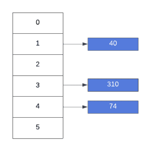
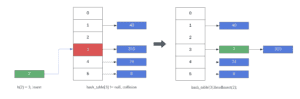
According to our function,  , 9 will be inserted at index 5, whereas the last item, 2 will be inserted at index 3:
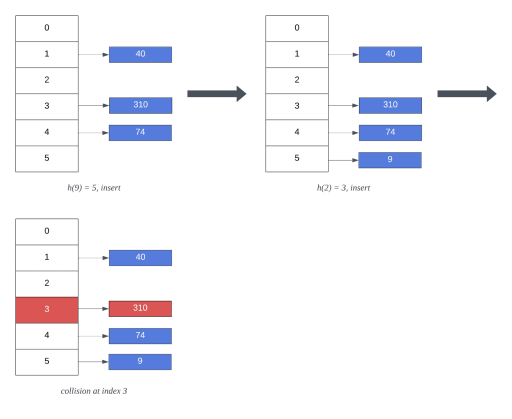
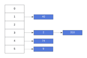
Once we try to insert 2, we encounter a collision with key 310. However, because we’re using separate chaining as our collision resolution algorithm, our hash table results in the following state after inserting all elements in :
Let’s dive into the separate chaining algorithm and learn how we obtained the previous state in our hash table.
To use the separate chaining technique, we represent hash tables as a list of linked lists. In other words, every index at the hash table is a hash value containing a chain of elements.
Once a collision happens, inserting a key into a list at a particular index could be costly. That is, if we disallow duplicate keys, we must search throughout the entire list first. Yet, if we allow duplicate elements, we optimize the process by inserting them at the head of the list. On the other hand, searching for an element involves traversing through the entire list until the key is found.
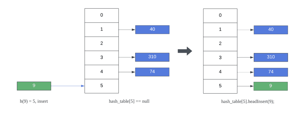
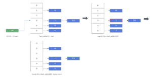
Let’s walk through the algorithm using as the input set and a hash table with the following initial state:

Currently, there are no elements at index 5. Therefore, inserting 9 involves creating a new linked list with a single element. Subsequently, new keys mapping to the same index will be added to the list:
Next, inserting 2 at index 3 results in a collision. In other words, there is an existing list at index 3 storing other values. In this case, separate chaining simply inserts the key at the beginning of the list. As a result, the list at index 5 now contains 2 keys and each element still maps to its original hash index:
Note that we never checked for duplicate elements in the previous insert operations. Both previously inserted keys could have been in the hash table already. Nonetheless, to disallow duplicate elements, we must search for the key before inserting it.
Let’s look at an example where we try to insert 40, and we disallow duplicate keys in our hash table. For simplicity’s sake, we’ll use the final state of our previous example:
In our previous example, we searched and tried to insert an existing element into our hash table. As a result, no insert operation was performed.
Overall, in separate chaining, keys will use the same index they originally generated from the hash function. This advantage allows searching for a key more performant if we have a good hash function that distributes the elements fairly across the has table.
Let’s look at the pseudocode for separate chaining For simplicity’s sake, we’ll use two different functions to determine whether a key can be inserted or found in the hash table. Let’s start with the insert operation.
The insert implementation is a void function that adds the key to their corresponding list. The following function creates a new linked list if one does not exist at the specified index.
However, if the list already exists, we simply add the new element:
function Insert(hash_table, key, hash_value):
    // INPUT
    //     hash_table = hash table data structure
    //     key = key to insert
    //     hash_value = computed hash value for the key
    // OUTPUT
    //     Inserts a key into the hash table using separate chaining

    if hash_table[hash_value] = null:
        hash_table[hash_value] <- new LinkedList(key)
    else:
        hash_table[hash_value].headInsert(key)
Note that if the Insert function is called multiple times with the same key value, the list will contain duplicates. Next, let’s look at a different implementation to disallow duplicate elements in our hash table:
function InsertNoDuplicates(hash_table, key, hash_value):
    // INPUT
    //     hash_table = hash table data structure
    //     key = key to insert
    //     hash_value = computed hash value for the key
    // OUTPUT
    //     Inserts a key into the hash table only if it's not already present

    if Search(hash_table, key, hash_value) != -1:
        return
    if hash_table[hash_value] = null:
        hash_table[hash_value] <- new LinkedList(key)
    else:
        hash_table[hash_value].headInsert(key)
This time, we call the Search function first to determine whether the key value is already in the list. Conversely, if key is not part of the list, we use the same Insert logic from the previous example.
The search implementation is a function that returns the index at which we find the key in the list. If the key is not in the hash table, we return -1. In this function, we loop through the list at the index generated by the hash function until we find the key or reach the end.
Let’s look at the pseudocode for search:
function Search(hash_table, key, hash_value):
    // INPUT
    //     hash_table = hash table data structure
    //     key = key to search for
    //     hash_value = computed hash value for the key
    // OUTPUT
    //     index of the key in the list if found, -1 otherwise

    list <- hash_table[hash_value]
    for i <- 0 to list.length - 1:
        if list.get(i) = key:
            return i
    return -1
The Search algorithm expects a hash_value parameter, representing the index at which we’ll search for the key value. At this index, we refer to the list of all elements mapping to this location in the hash table.
Finally, we iterate through every element until our loop finds key or reaches the end of the list.
In separate chaining, we can achieve a constant  insert operation for all new elements in a hash table. That is, if we allow duplicate elements, then separate chaining guarantees a constant runtime for insertions. Yet, preventing duplicate keys in the table requires a
  traversal before adding a new element to ensure it’s not already in the list.
That said, traversing through the list is a linear operation, and as a consequence, searching using separate chaining has a time complexity.
In this article, we learned about the separate chaining technique. This algorithm leverages linked lists to resolve collisions when multiple keys have the same hash value. Further, we covered all algorithm steps and analyzed how the time complexity differs from insertion and search.
Separate chaining is a useful technique for implementing hash tables, particularly when duplicate keys are not allowed, yielding an runtime for all insertions.