

Yes, we're now running our only Summer Sale. All Courses are 30% off until 20th July, 2026:
Learn through the super-clean Baeldung Pro experience:
>> Membership and Baeldung Pro.
No ads, dark-mode and 6 months free of IntelliJ Idea Ultimate to start with.
1. Introduction
In this tutorial, we’ll learn about linear probing – a collision resolution technique for searching the location of an element in a hash table.
Generally, hash tables are auxiliary data structures that map indexes to keys. However, hashing these keys may result in collisions, meaning different keys generate the same index in the hash table.
We’ll demonstrate how linear probing helps us insert values into a table despite all collisions that may occur during the process. Additionally, we’ll look at how linear probing works for search operations.
2. Linear Probing
Linear probing is one of many algorithms designed to find the correct position of a key in a hash table. When inserting keys, we mitigate collisions by scanning the cells in the table sequentially. Once we find the next available cell, we insert the key. Similarly, to find an element in a hash table, we linearly scan the cells until we find the key or all positions have been scanned.
Hence, before diving into the details of the algorithm, let’s demonstrate different scenarios of hashing keys and collisions. First, let’s assume we have the following set of keys  and an arbitrary hash function
  that yields the following:

Furthermore, suppose our hash table has an arbitrary length of 6, and we want to insert the remaining elements of  :
:
: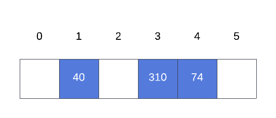
Thus, according to our function,  , 9 will be inserted at index 5, whereas the last item in the set that is 2 will be inserted at index 3:
, 9 will be inserted at index 5, whereas the last item in the set that is 2 will be inserted at index 3: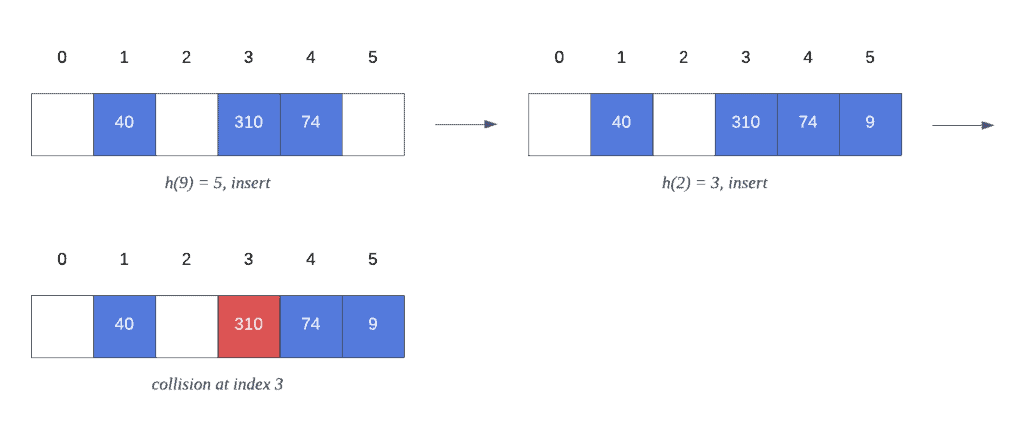
Once we try to insert 2 into our hash table, we encounter a collision with key 310. However, because we’re using linear probing as our collision resolution algorithm, our hash table results in the following state after inserting all elements in :
: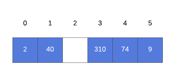
Now, let’s dive into the linear probing algorithm and learn how we obtained the previous state in our hash table.
3. Algorithm
To use the linear probing algorithm, we must traverse all cells in the hash table sequentially. Hence, inserting or searching for keys could result in a collision with a previously inserted key. Yet, with linear probing, we overcome this by searching linearly for the next available cell.
Furthermore, let’s walk through the algorithm using as the input set and a hash table with the following initial state:
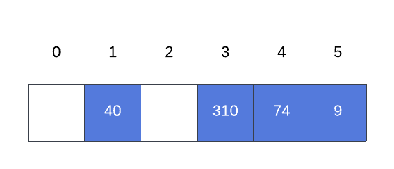
As we saw previously, inserting 2 into the hash table results in a collision at index 3. Therefore, we must visit every cell on the table from left to right, looking for an empty space. Let’s look at this process closely:
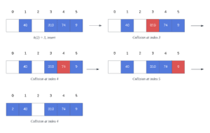
When trying to insert 2 into the table, we encounter three collisions during the process. Thus, the first collision occurs at index 3, which is the hash value generated by the function for this particular key. However, the cell at index 3 is not empty, and we continue to the next cell. Hence, cells #4 and #5 are also occupied by other keys, and we reached the end of the hash table.
Ultimately, because we have not checked the cells preceding index 3, we must loop all the way around to the beginning of the hash table. Consequently, the key 2 is inserted at index 0, given that it was the next available space.
Moreover, there is one more case we still need to consider. That is, what if the hash table has no capacity? Then, the linear probing algorithm must have a way to terminate the loop scanning the cells. We’ll demonstrate this in the pseudocode section.
Similarly, instead of inserting, searching for 2 leads to the same iterations we covered when inserting the key.
4. Pseudocode
Let’s look at the pseudocode for linear probing. For simplicity’s sake, we’ll use two different functions to determine whether a key can be inserted or found in the hash table. Thus, let’s start with the insert operation.
The insert implementation entails a function that returns a boolean value, indicating whether we can find a cell to insert our key:
algorithm LinearProbingInsert(hash_table, table_length, key, hash_value):
    // INPUT
    //    hash_table = the hash table to insert the key into
    //    table_length = the length of the hash table
    //    key = the key to insert
    //    hash_value = the initial hash value for the key
    // OUTPUT
    //    true if the key is successfully inserted, false if there is no space to insert the key

    index <- hash_value
    first_scan <- true

    while isEmpty(hash_table, index) = false:
        index <- (index + 1) mod table_length
        if index = hash_value and first_scan = false:
            return false
        first_scan <- false

    hash_table[index] <- key
    return true
Thus, the first step is to compute the initial index and set it as the start index. Additionally, we use an auxiliary isEmpty function to determine whether the cell at the current index is empty. If the cell isn’t empty, we move to the next index using linear probing. Additionally, we cover the case when the hash table has been fully scanned without finding an empty slot. If the hash table is full, it can’t accommodate the new keys.
Furthermore, as soon as we find an empty slot while scanning the hash table, we insert the key into that specific index.
Finally, the pseudocode returns true after successful insertion.
4.2. Search
To search an element in a hash table using linear probing, we use a similar approach to the insert operation. However, this time we return the index at which we find the key, or -1 when it’s not in the hash table. Additionally, the loop will continue if the element at the current index is not equal to the key.
Let’s look at the pseudocode for search:
algorithm LinearProbingSearch(hash_table, table_length, key, hash_value):
    // INPUT
    //    hash_table = the hash table to search in
    //    table_length = the length of the hash table
    //    key = the key to search for
    //    hash_value = the hash value of the key
    // OUTPUT
    //    the index where the key is found, or -1 if the key is not in the hash table

    index <- hash_value
    first_scan <- true

    while hash_table[index] != key:
        index <- (index + 1) mod table_length
        if index = hash_value and first_scan = false:
            return -1
        first_scan <- false

    return index
5. Time Complexity
A well-designed hash function and a hash table of size n increase the probability of inserting and searching a key in constant time. However, no combination between the two can guarantee a  operation.
Therefore, a collision causes linear probing to search linearly for the next available cell. Hence, given that our table size is n, we can infer that the maximum number of iterations is also n. Therefore, we can conclude that the time complexity for linear probing is  .
.
6. Conclusion
In this article, we learned about the linear probing technique. Furthermore, we use this algorithm to resolve collisions when multiple keys have the same hash value. Additionally, we covered all algorithm steps and analyzed their runtime complexity.
Finally, despite other alternatives to minimize collisions in a hash table, linear probing provides a solution and a simple implementation to code.