

Learn through the super-clean Baeldung Pro experience:
>> Membership and Baeldung Pro.
No ads, dark-mode and 6 months free of IntelliJ Idea Ultimate to start with.
Learn through the super-clean Baeldung Pro experience:
>> Membership and Baeldung Pro.
No ads, dark-mode and 6 months free of IntelliJ Idea Ultimate to start with.
In this tutorial, we’ll discuss the problem of finding the diameter of a graph. We’ll start by explaining what the problem is and then move on to algorithms for solving it. Finally, we’ll provide pseudocode for one algorithm and analyze its time complexity.
The diameter of a graph is defined as the largest shortest path distance in the graph. In other words, it is the maximum value of  over all
  pairs, where
  denotes the shortest path distance from vertex
  to vertex
  .
.
Alternatively, we can define the diameter in terms of vertex eccentricities. The eccentricity of a vertex , denoted by  , equals the maximum shortest path distance from to any other vertex. Then the diameter can be defined as the maximum of all vertex eccentricities.
If the input graph represents a transportation or road network, computing the diameter gives us a good idea of how far a vehicle will have to travel from one point to another in the worst case. Of course, this is assuming the vehicle can always take the shortest path from point  to point
  .
.
Here we illustrate the concept of diameter on an undirected graph (the diameter is marked with red):
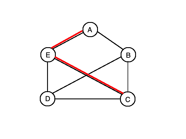
Let’s compute the diameter of the above graph. For the shortest path distances we have  ,
,  ,
,  ,
,  ,
,  ,
,  ,
,  ,
,  ,
,  , and
, and  . Therefore, our diameter is equal to
  since that is the maximum of these values.
The high-level strategy of the algorithms presented in this section is to compute all the shortest paths, keeping track of the maximum value seen so far. Then in the end we return the final maximum value as the diameter.
What if the input graph is a weighted directed graph with nonnegative edge weights? One approach we could take is to run Dijkstra’s algorithm from every vertex and keep track of the largest shortest path distance.
A better approach is to run an optimal all-pairs shortest paths algorithm such as the Floyd-Warshall algorithm. The advantage of this approach is that it uses less space and is easier to implement. In addition, it will work even if there exist negative edge weights in the graph whereas the Dijkstra approach will only work with nonnegative edge weights. Note that this Floyd-Warshall method can only be used if there are no negative cycles in the input graph.
If the graph is an undirected unweighted graph, we have a couple of options. One option is to run a breadth-first search from every vertex, keeping track of the maximum shortest path distance. Another option would be to first convert the graph to a directed graph with all edge weights equal to one, and then use the above mentioned Floyd-Warshall approach.
So, let’s look at some pseudocode for the Floyd-Warshall approach on a weighted directed graph without negative cycles:
algorithm FloydWarshall(M):
    // INPUT
    //    M = a matrix representing the edge weights of a directed graph G without negative cycles
    // OUTPUT
    //    Diameter = the diameter of G

    n <- length of M
    d <- create a three-dimensional array of size n times n times n
    d[0] <- M

    for k <- 1 to n:
        for i <- 1 to n:
            for j <- 1 to n:
                d[k, i, j] <- min(d[k-1, i, j], d[k-1, i, k] + d[k-1, k, j])

    Diameter <- d[n, 1, 1]

    for i <- 1 to n:
        for j <- 1 to n:
            if d[n, i, j] > Diameter:
                Diameter <- d[n, i, j]

    return Diameter
The above algorithm takes as input an  by matrix
  representing a weighted directed graph without negative cycles and outputs its diameter. An entry of this matrix,
  , equals:
 equals
 if does not equal and exists, and does not equal and does not exist
The first part of the algorithm is the same as the Floyd-Warshall algorithm. We define a matrix  which stores the values of the shortest paths between every pair of nodes.
More precisely, this matrix stores values ![d[k][i][j]](/wp-content/ql-cache/quicklatex.com-bb831f1db0c814120e5265ab1e4c1512_l3.svg "Rendered by QuickLaTeX.com") which represents the length of the shortest path from node to node which uses only vertices from the set
which represents the length of the shortest path from node to node which uses only vertices from the set  as its intermediate vertices. Then we have a triply nested loop which is a bottom-up dynamic programming procedure for filling out the values of the matrix .
Once we have computed all the shortest path values we compute the maximum value amongst all the ![d[n][i][j]](/wp-content/ql-cache/quicklatex.com-b3192269baa2e0ae1165b389660ccfc4_l3.svg "Rendered by QuickLaTeX.com") ‘s by iterating through every
‘s by iterating through every  pair and keeping track of the maximum value so far. This value is then returned as the diameter.
No matter which approach we take to computing the diameter of a graph, we are always going to end up with a worst-case complexity of  , where is the number of nodes in the graph.
This includes the Floyd-Warshall method. In the Floyd-Warshall approach, we first have a triple nested for loop with a constant time operation, which takes time. Then we have a double nested for loop which takes  time. Since dominates , our overall time complexity is .
In this article, we’ve seen that we can compute the diameter of a graph in time, where equals the number of nodes in the graph.
We’ve also seen pseudocode for the Floyd-Warshall approach and analyzed its time complexity.