

Learn through the super-clean Baeldung Pro experience:
>> Membership and Baeldung Pro.
No ads, dark-mode and 6 months free of IntelliJ Idea Ultimate to start with.
Learn through the super-clean Baeldung Pro experience:
>> Membership and Baeldung Pro.
No ads, dark-mode and 6 months free of IntelliJ Idea Ultimate to start with.
In this tutorial, we’ll discuss the problem of counting the number of shortest paths between two nodes in a graph. Firstly, we’ll define the problem and provide an example that explains it.
Secondly, we’ll discuss two approaches to this problem. The first one is for unweighted graphs, while the other approach is for weighted ones.
Suppose we have a graph  of
of  nodes numbered from
  to . In addition, we have
  edges that connect these nodes. We’re given two numbers
  and
and  that represent the source node’s indices and the destination node, respectively.
Our task is to count the number of shortest paths from the source node to the destination .
Recall that the shortest path between two nodes  and
and  is the path that has the minimum length among all possible paths between and .
Let’s check an example for better understanding. Suppose we have the following graph and we’re given  and
and  :
:
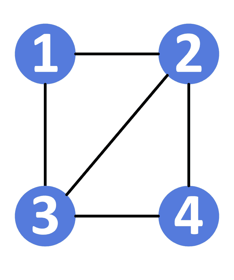
To go from node to node we have  paths:
 , with length equal to
  .
. , with length equal to
  .
. , with length equal to .
 , with length equal to .
As we can see, the shortest path has a length equal to . Also, we notice that we have two paths having a length equal to . Therefore, there are shortest paths between node and node .
The main idea here is to use BFS (Breadth-First Search) to get the source node’s shortest paths to every other node inside the graph. We’ll store for every node two values:
 : representing the length of the shortest path from the source to the current one.
 : representing the number of these shortest paths.
Initially, the value for all nodes is infinity except the source node equal to  (length of the shortest path from a node to itself always equal to
  ). Also, the value for all nodes is except the source node equal to (a node has a single shortest path to itself).
Next, we start traversing the graph using the BFS algorithm. Each time when we want to add a child of the current node to the queue, we’ll have two choices:
![\boldsymbol{ distance [child] > distance[current] + 1 }](/wp-content/ql-cache/quicklatex.com-69ed5805e3403ed85bfa690f66f7e8d3_l3.svg "Rendered by QuickLaTeX.com") , that means there is a path that goes from the source node to the child node with a smaller length than the previous path we have. So, we’ll minimize the child node’s distance value to be equal to the current node distance plus one. In addition, the value for the child node will be updated to be equal to the value of the current node.
, that means there is a path that goes from the source node to the child node with a smaller length than the previous path we have. So, we’ll minimize the child node’s distance value to be equal to the current node distance plus one. In addition, the value for the child node will be updated to be equal to the value of the current node.![\boldsymbol{ distance [child] = distance [current] + 1 }](/wp-content/ql-cache/quicklatex.com-2fbcb88c959f130ce82223a95abb13c1_l3.svg "Rendered by QuickLaTeX.com") , that means all the shortest paths that go from the source node to the current node will be added to the number of shortest paths of the child node. The reason is that they will have the same length as the shortest path of the child node after adding the edge that connects
, that means all the shortest paths that go from the source node to the current node will be added to the number of shortest paths of the child node. The reason is that they will have the same length as the shortest path of the child node after adding the edge that connects  with its
  . So, we’ll keep the distance value of the child node the same. However, we’ll increase the value of the child node by the value of the current node.
Finally, the value of the node will have the number of shortest paths that go from the source node to the destination node . Also, the distance value of the node will have the length of the shortest path that goes from to .
Let’s take a look at the implementation:
algorithm BFSApproachForUnweightedGraphs(V, G, S, D):
    // INPUT
    //     V = the number of nodes in the graph
    //     G = the graph stored as an adjacency list
    //     S = the index of the source node
    //     D = the index of the destination node
    // OUTPUT
    //     Returns the number of shortest paths between S and D

    distance <- map[v : infinity | v in V]
    paths <- map[v : 0 | v in V]
    queue <- create an empty queue
    queue.add(S)
    distance[S] <- 0
    paths[S] <- 1

    while queue is not empty:
        current <- queue.front()
        queue.pop()
        for child in G[current]:
            if visited[child] = false:
                queue.add(child)
                visited[child] <- true
            if distance[child] > distance[current] + 1:
                distance[child] <- distance[current] + 1
                paths[child] <- paths[current]
            else if distance[child] = distance[current] + 1:
                paths[child] <- paths[child] + paths[current]

    return paths[D]
Initially, we declare two arrays:
: where ![distance[u]](/wp-content/ql-cache/quicklatex.com-1fa1e0ad8b95956921f58789210256f3_l3.svg "Rendered by QuickLaTeX.com") represents the length of the shortest path that goes from the source node to the node
represents the length of the shortest path that goes from the source node to the node  .: where
 ![paths[u]](/wp-content/ql-cache/quicklatex.com-7e81975fc3d1e6a88c88b7ab7d20cbe0_l3.svg "Rendered by QuickLaTeX.com") represents the number of shortest paths from the source node to the node .
represents the number of shortest paths from the source node to the node .We also declared an empty queue to store nodes during BFS traversal.
Next, we perform multiple steps as long as the queue isn’t empty. In each step, we take the node positioned in the front of the queue and iterate over its children. For each child, we check whether we haven’t visited that node before. If so, we add it to the queue and mark it as a visited node. Also, we update the and value for the node based on the rules mentioned in section 3.1.
Finally, we return ![paths[D]](/wp-content/ql-cache/quicklatex.com-21adf166821683b88d5bbfacc37fc997_l3.svg "Rendered by QuickLaTeX.com") which stores the number of shortest paths that go from the source node to the destination.
which stores the number of shortest paths that go from the source node to the destination.
The complexity of this approach is the same as the BFS complexity, which is  , where is the number of nodes and is the number of edges. The reason behind this complexity is that we iterate over each node only once. Therefore, we iterate over its children once. In total, we iterate over each edge once as well.
We’ll apply the same concepts from the BFS Approach to solve the same problem for weighted graphs. However, to get the shortest path in a weighted graph, we have to guarantee that the node that is positioned at the front of the queue has the minimum distance-value among all the other nodes that currently still in the queue. So, we’ll use Dijkstra’s algorithm.
In Dijkstra’s algorithm, we declare a priority queue that stores a pair of values:
 : representing the length of the path we took from the source node to the current one.
 : representing the current node itself.
We’ll set the priority of our queue to give us the with the minimal to get the shortest path from the source node to the current node.
Finally, the remaining workflow will still the same as the BFS Approach.
Let’s take a look at the implementation:
algorithm DijkstrasApproachForWeightedGraphs(G, S, D):
    // INPUT
    //     V = the number of nodes in the graph
    //     G = the graph stored as an adjacency list
    //     S = the index of the source node
    //     D = the index of the destination node
    // OUTPUT
    //     Returns the number of shortest paths between S and D

    distance <- [n in V | infinity]
    paths <- [n in V | 0]
    priority_queue <- create an empty priority queue
    priority_queue.add({0, S})
    distance[S] <- 0
    paths[S] <- 1

    while priority_queue is not empty:
        current <- priority_queue.front().node
        length <- priority_queue.front().length
        priority_queue.pop()

        for edge in G[current]:
            node <- edge.node
            cost <- edge.cost

            if distance[node] > distance[current] + cost:
                priority_queue.add((length + cost, node))
                distance[node] <- distance[current] + cost
                paths[node] <- paths[current]
            else if distance[node] = distance[current] + cost:
                paths[node] <- paths[node] + paths[current]

    return paths[D]
Initially, we declare the same two arrays from the previous approach:
: where represents the length of the shortest paths from the source node to the node .: where represents the number of shortest paths from the source node to the node .We also declare an empty priority queue to store the explored nodes and sorted them in acceding order according to their distance value.
Next, we perform similar steps to the ones in unweighted graphs. As long as the priority queue isn’t empty, we pop the node positioned in the front of the priority queue with its (length of the path we took from the source node to the current node).
After that, we iterate over the children of the current node. For each child, we check whether it has a distance value greater than the current node’s distance value plus the cost of the current-child edge. If so, we add this child to the priority queue. Also, we update the value and value for the child node.
In the case of weighted graphs, the next steps are tweaked a little:
![\boldsymbol{ distance [child] > distance [current] + cost }](/wp-content/ql-cache/quicklatex.com-c3e806d3596366170bdfc8d9a2353a8e_l3.svg "Rendered by QuickLaTeX.com") , we minimize the distance value of the child node to be equal to the current node distance plus the cost of the current-child edge. In addition, the value for the child node will be updated to be equal to the value of the current node.
, we minimize the distance value of the child node to be equal to the current node distance plus the cost of the current-child edge. In addition, the value for the child node will be updated to be equal to the value of the current node.![\boldsymbol{ distance [child] = distance [current] + cost }](/wp-content/ql-cache/quicklatex.com-eeea0f1ca28e2a285095b17b03f7451e_l3.svg "Rendered by QuickLaTeX.com") , we keep the distance value of the child node the same. Also, we increase the value of the child node by the value of the current node.
, we keep the distance value of the child node the same. Also, we increase the value of the child node by the value of the current node.Finally, we return ![paths [D]](/wp-content/ql-cache/quicklatex.com-29cdba036196a901a714656318f5fba8_l3.svg "Rendered by QuickLaTeX.com") which store the number of shortest paths that go from the source node to the destination node.
which store the number of shortest paths that go from the source node to the destination node.
The complexity here is the same as the Dijkstra complexity, which is  , where is the number of nodes and is the number of edges. The reason is similar to the BFS approach. Since we iterate over each edge once and the priority queue needs
  complexity to add each node, then
  is the time complexity to keep all the nodes in the priority queue sorted by their length value.
In this tutorial, we presented the problem of counting the number of shortest paths between two nodes in a graph. We explained the general idea and discussed two approaches for the weighted and unweighted graphs.