An Introduction to Generative Adversarial Networks

1. Overview

In this tutorial, we’ll introduce Generative Adversarial Networks (GANs).

First, we’ll introduce the term generative models and their taxonomy. Then, a description of the architecture and the training pipeline of a GAN will follow, accompanied by detailed examples. Finally, we’ll talk about the challenges and the applications of GANs.

2. Generative Models

In Machine Learning, there are two major types of learning:

Supervised Learning where we are given the independent variables $\mathbf{X}$ and the corresponding label $\mathbf{Y}$ and our goal is to learn a mapping function $\mathbf{f: X \to Y}$ that minimizes a predefined loss function. In these tasks, we train discriminative models that aim to learn the conditional probability $p(Y|X)$ . Examples of supervised learning tasks include classification, regression, etc.

Unsupervised Learning where we are given only the independent variables $\mathbf{X}$ and our goal is to learn some underlying patterns of the data. In these tasks, we train generative models that aim to capture the probability $p(X)$ . Examples of unsupervised learning tasks include clustering, dimensionality reduction, etc.

Generally, a generative model tries to learn the underlying distribution of the data. Then, the model is able to predict how likely a given sample is and to generate some new samples using the learned data distribution.

There are two types of generative models:

On the one hand, we have the explicit density models that assume a prior distribution of the data. Here, we define an explicit density function, and then we try to maximize the likelihood of this function on our data. If we can define this function in a parametric form, we talk about a tractable density function. However, in many cases like images, it is impossible to design a parametric function that captures all the data distribution, and we have to use an approximation of the density function.

On the other hand, there are the implicit density models. These models define a stochastic procedure that directly generates data. GANs fall into this category:

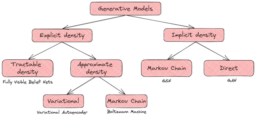
Above, we can see the taxonomy of generative models as proposed by Ian Goodfellow.

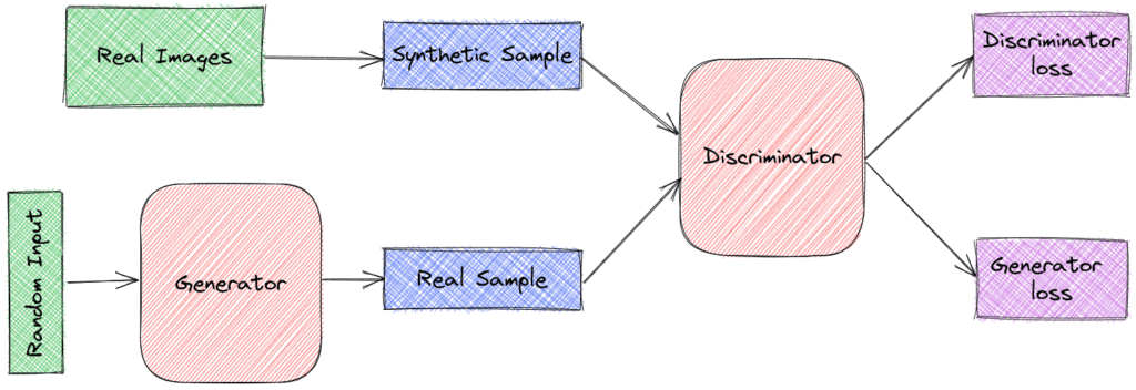
3. Generative Adversarial Networks

3.1. Architecture

Let’s start with the basic architecture of a GAN that consists of two networks.

First, there is the Generator that takes as input a fixed-length random vector $z$ and learns a mapping $G(z)$ to produce samples that mimic the distribution of the original dataset

Then, we have the Discriminator that takes as input a sample $x$ that comes either from the original dataset or from the output distribution of the Generator. It outputs a single scalar that represents the probability that $x$ came from the original dataset

Both $G$ and $D$ are differentiable functions that are represented by neural networks.

3.2. Loss Functions

We can think of $\mathbf{G}$ as a team of counterfeiters that produce fake currency while we can compare $\mathbf{D}$ to the police that tries to detect the counterfeit currency. The goal of $G$ is to deceive $D$ and use the fake currency without getting caught. Both parties try to improve their methods until, at some point, the fake currency cannot be distinguished from the genuine one.

More formally, $\mathbf{D}$ and $\mathbf{G}$ play a two-player minimax game with the following objective function:

$\mathbf{min_G \ max_D \ log D(x) + log (1 - D(G(z)))}$

where $x$ comes from the original dataset and $z$ is the random vector.

We observe that the objective function is defined using both models’ parameters. The goal of $G$ is to minimize the term $log (1 - D(G(z)))$ in order to fool the discriminator in classifying the fake samples as real ones.

In parallel, the goal of $D$ is to maximize $log D(x) + log (1 - D(G(z)))$ that corresponds to the probability of assigning the correct label to both the real samples and the samples from the generator.

It is important to note here that this is not a usual optimization problem since each model’s objective function depends on the other model’s parameters, and each model controls only its own parameters. That’s why we talk about a game and not an optimization problem. While the solution to an optimization problem is a local or global minimum, the solution here is a Nash equilibrium.

3.3. Training

Simultaneous SGD is used for training a GAN. In each step, we sample two batches of:

$x$ samples from the original dataset
$z$ vectors from the prior random distribution

Then, we pass them through the respective models as in the previous figure. Finally, we apply two gradient steps simultaneously: one that updates the parameters of $G$ in respect to its objective function and one that updates the parameters of $D$ .

3.4. DCGAN

One of the most well-known GAN architectures for images is the Deep Convolutional GAN (DCGAN) which has the following characteristics. Batch normalization is applied in all the layers of the Generator and the Discriminator. Of course, their output layers are not normalized in order for them to learn the real mean and scale of the image distribution.

Then the Generator uses the convolutional architecture:

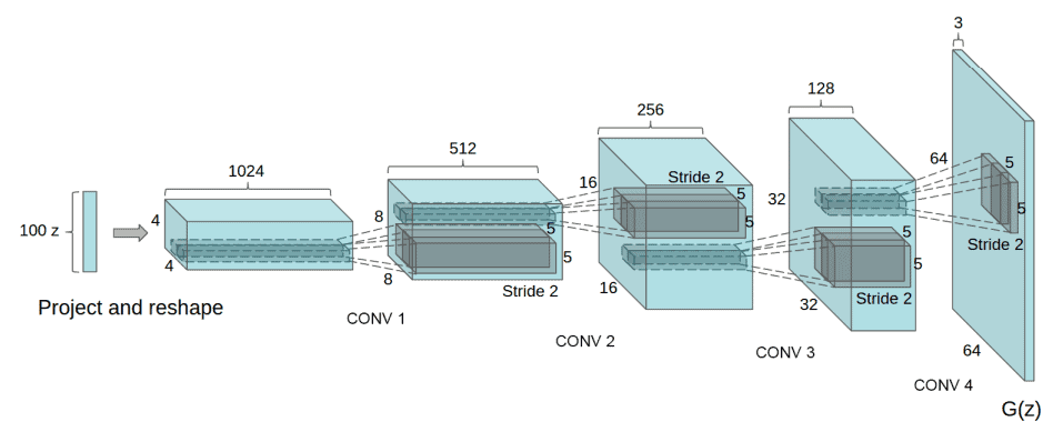
During training, Adam optimizer is used instead of SGD, which then uses ReLU activation in the Generator and Leaky ReLU activation in the discriminator.

3.5. Example

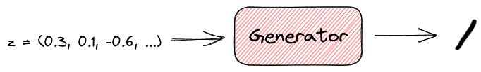
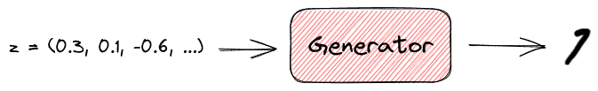
Now let’s describe how a GAN learns to generate images of the digit “7”.

First, the Generator samples a vector $z$ from some simple prior distribution and outputs an image $G(z)$ . Since the parameters of the model are randomly initialized, the output image is not even close to the digit “7”:

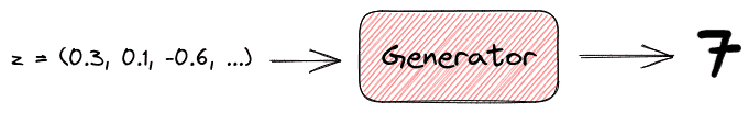
During training, the Generator learns to produce images closer and closer to the original distribution (that depicts the digit “7”) in order to fool the Discriminator. So, at some point $\mathbf{G}$ outputs images more similar to the digit “7”:

In the end, the image distribution of the output of the generator and the original distribution is very close to each other, and synthetic images depicting the digit “7” are generated:

4. Applications

Now let’s talk about some of the most useful applications of GANs.

4.1. Data Augmentation

GANs can be used to generate synthetic samples for data augmentation in cases where the provided data are limited.

4.2. Image Inpainting

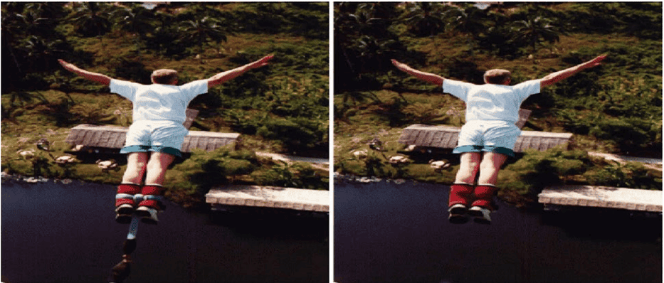
There are many cases where we want to reconstruct an image and either remove unwanted objects or restore damaged portions of old images. GANs have achieved excellent results in this task, like the one below where the model removed the rope:

4.3. Super‑Resolution

This term refers to the procedure of generating a high-resolution image from a lower resolution one. It is a very useful task with many applications in security.

4.4. Image to Image Translation

Here we want to translate an input image into an output image, which is a common task in computer graphics and image processing. There are many GAN architectures that deal with this problem, like CycleGAN:

We mentioned just a few applications of these models. GANs can improve numerous tasks, and their applicability is not yet fully explored. Every year, we discover more and more areas where GANs can be proved useful.

5. Challenges

Although GANs have already succeeded in many areas, there are yet many challenges that we have to face when training a GAN for unsupervised learning.

5.1. Non-convergence

As we mentioned earlier, training a GAN is not an ordinary optimization problem but a minimax game. So, achieving convergence to a point that optimizes the objectives of both the generator and the discriminator is challenging since we have to learn a point of equilibrium. Theoretically, we know that simultaneous SGD converges if the updates are made in function space. When using neural networks, this hypothesis does not apply, and convergence is not theoretically guaranteed. Also, many times we observe cases where the Generator undoes the progress of the Discriminator without arriving anywhere useful and vice versa.

5.2. Evaluation

One important aspect of every learning task is evaluation. We can qualitatively evaluate a GAN quite easily by inspecting the synthetic samples that the generator produces. However, we need quantitative metrics in order to robustly evaluate any model. Unfortunately, it is not clear how to quantitatively evaluate generative models. Sometimes, models that obtain good likelihood generate unrealistic samples, and other models that generate realistic samples present poor likelihood.

5.3. Discrete Outputs

To train a GAN, the architecture of the generator should be differentiable. However, if we want the generator to produce discrete data, the respective function won’t be differentiable. Although there are many proposed solutions to this restriction, there is no optimal universal solution. Dealing with this problem will help us use GANs for domains like NLP.

5.4. Using the Code

The Generator takes as input a random vector $z$ and generates a sample $x$ . Therefore, the vector $z$ can be considered as a feature representation of the sample $x$ and can be used in a variety of other tasks. However, it is very difficult to obtain $\mathbf{z}$ given a sample $\mathbf{x}$ since we want to move from a high-dimensional space to a low-dimensional one.

6. Conclusion

In this tutorial, we made an introduction to GANs. First, we talked about the general field of generative models presenting a proposed taxonomy. Then, we described the basic architecture and training procedure of a GAN. Finally, we briefly mentioned the applications and the challenges of GANs.

Full Archive

About Baeldung

Core Concepts

Operating Systems

Artificial Intelligence

Graph Theory

Latex