

Learn through the super-clean Baeldung Pro experience:
>> Membership and Baeldung Pro.
No ads, dark-mode and 6 months free of IntelliJ Idea Ultimate to start with.
Learn through the super-clean Baeldung Pro experience:
>> Membership and Baeldung Pro.
No ads, dark-mode and 6 months free of IntelliJ Idea Ultimate to start with.
When implementing neural networks, activation functions play a role in determining the output of a neuron and, consequently, the model’s overall performance. They also impact the gradient flow. This means they can make training the network more or less difficult.
In this tutorial, we explain the GELU (Gaussian Error Linear Unit) activation function. We motivate its use, describe its implementation, and compare it with the standard ReLU activation function.
Activation functions are mathematical operations applied to the input of a neuron. Non-linearity is crucial for the network to learn complex mappings between inputs and outputs, enabling it to capture intricate patterns in the data. Common activation functions include the sigmoid, hyperbolic tangent (tanh), and rectified linear unit (ReLU).
Recent advancements have introduced novel functions that promise improved performance. The Gaussian Error Linear Unit (GELU) activation function is one such standout:
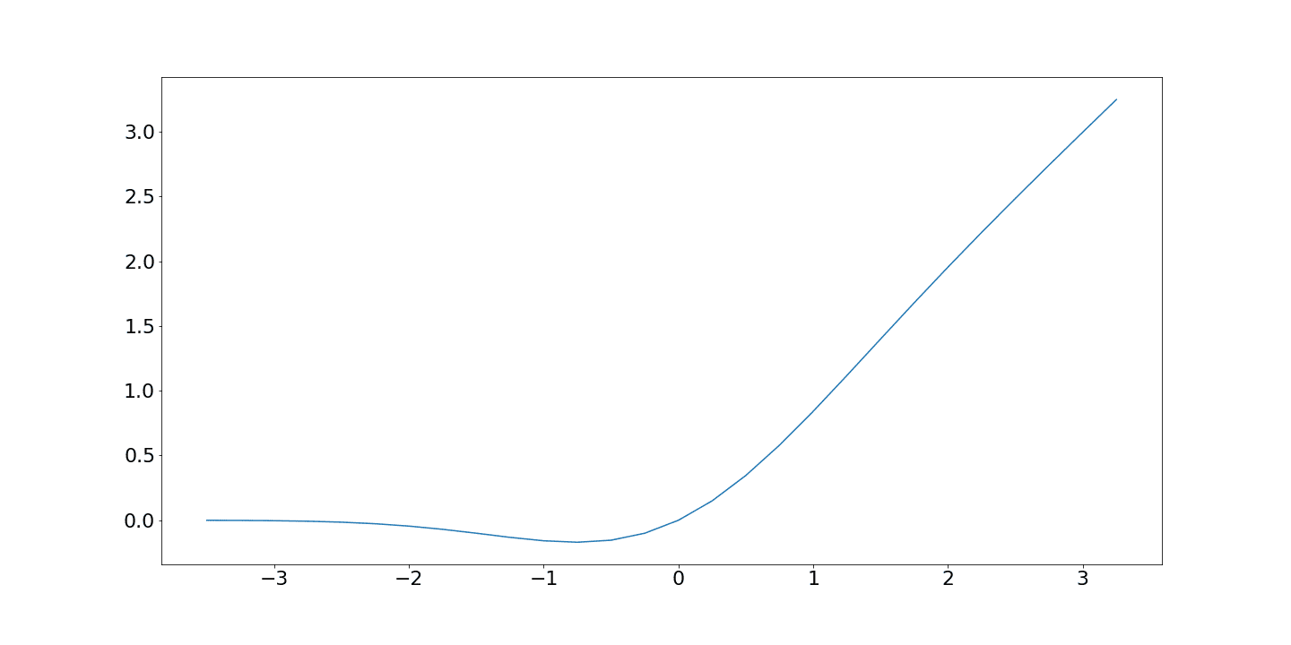
GELU, introduced by Dan Hendrycks and Kevin Gimpel in their 2016 paper “Gaussian Error Linear Units (GELUs),” has gained prominence for its ability to enhance the learning capabilities of neural networks. Unlike its predecessors, GELU is derived from a smooth approximation of the cumulative distribution function (CDF) of the standard normal distribution. It is our input times the standard normal CDF at that point:
![\[GELU(x) = x\times CDF(x) = x\times \frac{1}{2}\left(1 +erf \left(\frac{x}{\sqrt{2}}\right)\right)\]](/wp-content/ql-cache/quicklatex.com-e127521204d5c84848215293af73dbf4_l3.svg "Rendered by QuickLaTeX.com")
The erf is the Gaussian error function. It’s a well-supported function in many standard math and statistics libraries.
In its original formulation, GELU can’t be used in our neural networks as the function is complex and slow to compute.
Luckily, we can reformulate it:
![\[GELU_{\tanh}(x) = 0.5x \left(1 + \tanh\left(\sqrt{\frac{2}{\pi}}\left(x + 0.044715x^3\right)\right)\right)\]](/wp-content/ql-cache/quicklatex.com-0db6b867bd2f70799ec5ff0bcab0d5be_l3.svg "Rendered by QuickLaTeX.com")
Here, we approximate the Gaussian error function using the  function:
 introduces a linear component to the function applies the hyperbolic tangent function to the input, which helps maintain a smooth transition
 applies normalization, ensuring the output is within a reasonable range
There’s also a simpler sigmoid-based approximation:
![\[GELU_{\text{sigmoid}}(x) = x \times \text{sigmoid}(1.702\times x)\]](/wp-content/ql-cache/quicklatex.com-186c51d9da1c97d2e096242747ff4072_l3.svg "Rendered by QuickLaTeX.com")
These approximations are generally considered accurate, although the tails of and erf differ. In practice, the approximation functions well, and further refinement and more complex implementations are rarely necessary.
The benefits of the and sigmoid approximations are that they and their derivatives are easy to compute.
The key advantage of GELU lies in its smoothness and differentiability across the entire real line. This smoothness facilitates training, as gradient-based optimization algorithms can easily navigate the function’s landscape.
The smoothness also mitigates the problem of vanishing gradients. It occurs at or near the saturation point of the activation function, where changes to the input cease to impact the derivative. A smoother, more gradual gradient transition provides a more consistently informative training signal.
The smoothness also mitigates abrupt gradient changes found in other activation functions, aiding convergence during training.
The ReLU activation function has a hard cut-off at 0 for any negative number and otherwise produces a linear result. GELU follows a similar but smoother pattern:
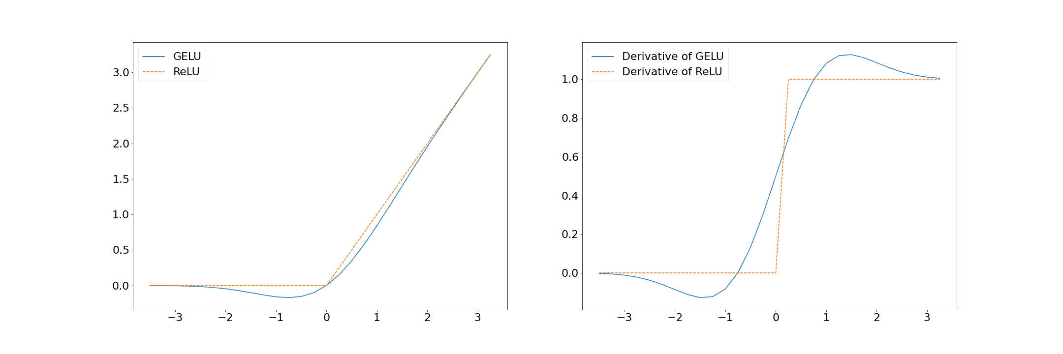
GELU has a significantly smoother gradient transition than the sharp and abrupt ReLU.
A further observation of the GELU function shows that it is non-monotonic. That is, it isn’t always increasing or decreasing. This feature allows GELU to capture more complex patterns in the data. The reasoning is that since it’s based on the normal cumulative density function, it may better capture Gaussian-like data.
There are a few reasons to favor GELU in deep neural networks. These range from improved smoothness to a greater capacity to capture non-linear relationships:
| GELU Pros | GELU Cons |
|---|---|
| Addresses the vanishing gradient with no dead neurons | Increased computational complexity |
| Smoothness across the full range of input values | Performance can be task-specific |
| Non-monotonic behavior can capture complex patterns | Reduced interpretability due to increased complexity |
Further, GELU has been shown to improve performance in transformer architectures and on standard benchmarks such as cifar-10 and is easy to include in models.
GELU is based on a Gaussian cumulative density function, so data exhibiting similar properties may be particularly suited to GELU models.
However, GELU increases computational complexity and is less interpretable. So, it’s important to remember these are empirical results, and we should evaluate whether or not GELU is the right choice for our particular task.
In this article, we explained the GELU activation function and compared it with the popular ReLU activation function. Further, we described its benefits and discussed cases where it offers improved performance. GELU provides a smooth, non-monotonic, and differentiable alternative to traditional activation functions.