

Yes, we're now running our only Summer Sale. All Courses are 30% off until 20th July, 2026:
Learn through the super-clean Baeldung Pro experience:
>> Membership and Baeldung Pro.
No ads, dark-mode and 6 months free of IntelliJ Idea Ultimate to start with.
1. Overview
In this tutorial, we’ll discuss the flood fill algorithm, also known as seed fill.
Firstly, we’ll define the algorithm and provide an example that explains it.
Secondly, we’ll discuss two approaches to this algorithm. Finally, we’ll show some useful usages of it.
2. Defining the Algorithm
Flood fill is an algorithm that determines the area connected to a given cell in a multi-dimensional array.
Suppose we have a colorful image that can be represented as a 2D array of pixels. Each pixel in this 2D array has a color. Our task is to change the color of some area that has a specific color to a new color.
Initially, the flood fill algorithm takes two parameters:
 : which represents the index of the cell that we want to recolor with all its connected cells that have the same initial color.
 : represents the new color that the given area will have after applying the flood fill algorithm.
For simplicity, we’ll consider the neighbors of each cell to be the cells to the top, bottom, left, and right of the cell. In addition, to consider a cell as a part of the connected area, it must have the same color as the initial one.
Let’s check an example for better understanding. Suppose we have the following 2D array:
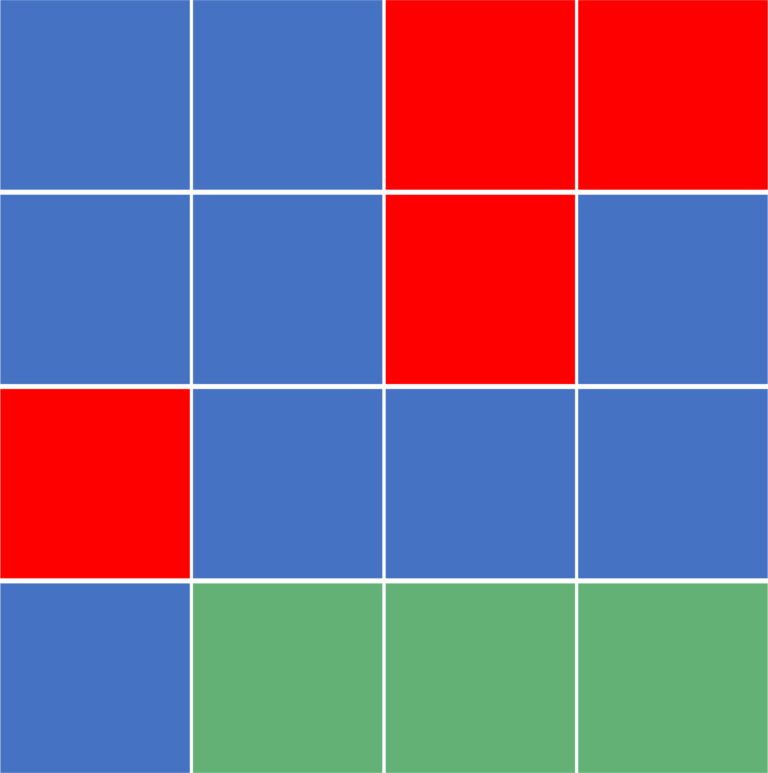
Suppose that we’re given  and
and  . As we can see the color of cell
  is blue. Therefore, we’ll recolor all its connected cells that have the same color to the
  :
:
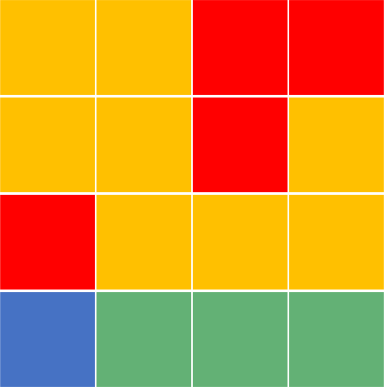
Note that we don’t only color the neighbors of the initial cell. In the contrast, we consider the neighbors of the initial cell, and keep finding the neighbors of each newly discovered cell. The operation continues until no new neighboring cells are discovered.
In addition, the bottom left cell still has a blue color at the end. The reason is that it’s not a part of the connected area that contains the initial cell.
3. BFS Approach
The main idea here is to use the BFS (Breadth-First Search) algorithm to traverse to the four adjacent cells of the  and recolor them. To do that, we’ll divide our implementation into three steps.
First, we’ll create a function that helps us decide whether a certain cell is valid to move to, or not. Secondly, we’ll implement the BFS approach. Finally, we’ll see how to improve the implementation to make it cleaner and shorter.
3.1. Validating a Neighboring Cell
Let’s take a look at the implementation:
algorithm isValid(row, column, color):
    // INPUT
    //    row = the row number of the cell
    //    column = the column number of the cell
    //    color = the color to check in the cell
    // OUTPUT
    //    Returns true if the cell is valid, false otherwise

    if row < 1 or row > the number of rows:
        return false
    if column < 1 or column > the number of columns:
        return false
    if G[row, column] != color or visited[row, column]:
        return false
    return true
The  function will tell us whether the cell we want to move to is valid or not. The
  is valid if the following conditions are true:
 the current row is inside the rows boundry.
 the current column is inside the columns boundry.
![\boldsymbol{ G [row] [column] = color }:](/wp-content/ql-cache/quicklatex.com-7fac07d8eaced54c03aada897b086c5f_l3.svg "Rendered by QuickLaTeX.com") the color of the cell equals to the color of the source cell.
the color of the cell equals to the color of the source cell.![\boldsymbol{ \neg visited [cell (row, column)] }:](/wp-content/ql-cache/quicklatex.com-db5e8d88fc5c8ba3ff927ee598b55231_l3.svg "Rendered by QuickLaTeX.com") we didn’t visit this cell before.
we didn’t visit this cell before.
3.2. Naive Implementation
Take a look at the first implementation of the BFS approach:
algorithm BFS(G, start_position, new_color):
    // INPUT
    //    G = the 2D array representing the grid
    //    start_position = the index of the starting cell
    //    new_color = the new color to be applied
    // OUTPUT
    //    The 2D array G with the specified area colored with new_color

    target_color <- G[start_position.row, start_position.column]

    visited <- initialize a 2D array with false values

    queue <- empty queue
    queue.add(start_position)

    visited[start_position.row, start_position.column] <- true
    G[start_position.row, start_position.column] <- new_color

    while queue is not empty:
        current <- queue.front()
        queue.pop()

        G[current.row, current.column] <- new_color

        if isValid(current.row + 1, current.column, target_color):
            queue.add(new Cell(current.row + 1, current.column))
            visited[current.row + 1, current.column] <- true
            G[current.row + 1, current.column] <- new_color
        if isValid(current.row - 1, current.column, target_color):
            queue.add(new Cell(current.row - 1, current.column))
            visited[current.row - 1, current.column] <- true
            G[current.row - 1, current.column] <- new_color
        if isValid(current.row, current.column + 1, target_color):
            queue.add(new Cell(current.row, current.column + 1))
            visited[current.row, current.column + 1] <- true
            G[current.row][current.column + 1] <- new_color
        if isValid(current.row, current.column - 1, target_color):
            queue.add(new Cell(current.row, current.column - 1))
            visited[current.row, current.column - 1] <- True
            G[current.row, current.column - 1] <- new_color
Initially, we declare an empty queue to store the cells during BFS traversal. Also, we declare  variable which represents the initial color of the source cell.
Next, we perform multiple steps as long as the queue isn’t empty. In each step, we take the  cell that is positioned in the front of the queue, remove it from the queue, change its color to the and mark it as a visited cell. After that, we add her adjacent valid neighbor cells to the queue.
Finally, when the  loop is finished, all the area of the initial cell will be marked as visited and has the new color.
3.3. Shorter Implementation
As we can see, our implementation is messy a little bit. So, to make it cleaner, we’ll declare two transition arrays that will help us move to all adjacent cells with a single line of code.
algorithm BFS(G, start_position, new_color):
    // INPUT
    //    G = the 2D array representing the grid
    //    start_position = the index of the starting cell
    //    new_color = the new color to be applied
    // OUTPUT
    //    The 2D array G with the specified area colored with new_color

    delta_x <- [+1, -1, 0, 0]
    delta_y <- [0, 0, +1, -1]

    target_color <- G[start_position.row, start_position.column]
    visited <- initialize a 2D array with false values

    queue <- an empty queue
    queue.add(start_position)

    visited[start_position.row][start_position.column] <- True

    while queue is not empty:
        current <- queue.front()
        queue.pop()
        G[current.row, current.column] <- new_color

        for i <- 1 to 4:
            next_row <- current.row + delta_x[i]
            next_column <- current.column + delta_y[i]
            if isValid(next_row, next_column, target_color):
                visited[next_row, next_column] <- true
                queue.add(new Cell(next_row, next_column))
The transition arrays here will give us the offset needed from the current cell to move to the adjacent cells. For example, transition  will give us the cell that lies on the left of the current cell.
In addition, we can change the color of a cell when we retrieve it from the queue, rather than changing each cell before adding it to the queue.
The complexity of this approach is the same as the BFS complexity, which is  , where
  is the number of rows in our 2D array and
  is the number of columns. The reason behind this complexity is that it’s similar to the original BFS complexity which is
  , where
  is the number of vertices and
  is the number of edges.
In our case, the number of vertices is  , and the number of edges is
  ), because each cell has four adjacent cells.
4. DFS Approach
In the DFS (Depth-First Search) algorithm, we’ll apply the same concepts from the previous BFS Approach to traverse to the four adjacent cells of the and recolor them. In addition, we’ll use the function defined in section 3.1 and the enhanced version of visiting the neighbors using the transition array.
Let’s take a look at the implementation:

Initially, we declare the same two transition arrays from the previous approach.
Next, each time we enter the  function we mark the current cell as a visited. Also, we change the color of the current cell to the .
Then, we iterate over the four adjacent neighboring cells. For each one, we’ll check whether it’s valid to move to. If so, we’ll call the function recursively on that cell.
At the end, all of the areas that are connected to the source cell and have the same color as the source cell will be colored with the .
The complexity of this approach is the same as the DFS complexity, which is , where is the number of rows in our 2D array and is the number of columns. The reason behind this complexity is the same as the one described in section 3.3.
5. Usage
Let’s discuss some cases where we might need to use the flood fill algorithm:
- It’s used in the bucket fill tool of the paint programs to fill connected, similarly-colored areas with a different color. We can notice that we only click on one pixel of the image, and all the cells of the connected area related to the clicked cell have their color changed into the new one.
- In games such as Go and Minesweeper for determining which pieces are cleared. Suppose we clicked on some cell of the grid which didn’t have a mine nor a number. In this case, the game will open all the cells that are empty and inside the same connected area. However, in this case, there’s one update to the algorithm which is to stop when we reach a cell that contains a number.
- Check whether two cells are inside the same connected area. For this usage, we can give a unique identifier for each connected area in advance. Later, when we receive a query about two cells inside the grid, we’ll only need to check their respective identifiers and see whether they match or not.
6. Conclusion
In this article, we presented the Flood Fill algorithm. We explained the general idea and discussed two approaches to solving the problem. Finally, we provided a fair usage of the algorithm in real-life problems.