How to Find an Area of Overlapping Rectangles

1. Introduction

This tutorial focuses on techniques to solve the overlapping rectangle problem. Our goal is to calculate the overlapping area of a given number of rectangles. As an example, we find applications in the field of microprocessor design. In microprocessor design, certain areas and wires are not allowed to intersect or are just allowed to intersect for a certain degree.

2. Problem Description

Firstly the problem seems very easy: We have a finite number of rectangles and want to calculate their overlap. Additionally, the rectangles have sides that are either parallel to the – or the -axes. The target is to simply calculate the area where the rectangles intersect, ignoring the geometry of the intersection:

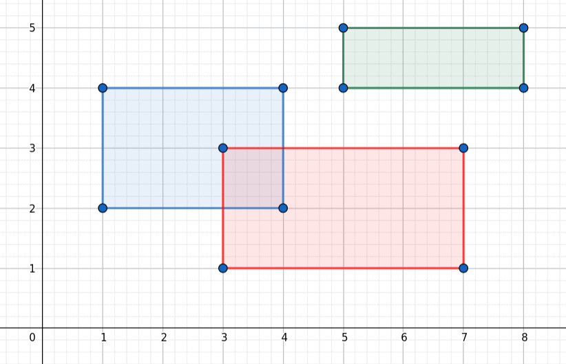
In our example, we see three rectangles. Only the red and the blue overlap. Furthermore, we want to calculate their shared area which is 1.

3. A Simple Solution

A simple solution would be to compare simply two rectangles with each other at one time, seeing which areas overlap.

3.1. Theoretic Approach

We realize this by creating intervals from their sides. One in the x-direction and one in the y-direction, meaning two intervals for each rectangle. Then we calculate the intersection of the two x-direction intervals as well as the y-direction ones. The two intersections combined create the two sides for the rectangle overlap.

3.2. Implementation

algorithm CalculateOverlap(l):
    // INPUT
    //    l = a list of rectangles
    // OUTPUT
    //    a = the area of overlap

    n <- the length of l
    a <- 0

    for i <- 0 to n:
        for j <- 0 to n:
            if i != j:
                a <- a + Compare(l[i], l[j])

    return a

algorithm Compare(R1, R2):
    // INPUT
    //    R1, R2 = two rectangles defined by two points A and B
    // OUTPUT
    //    a = the area of Overlap

    X <- 0
    Y <- 0 if R2.A.x > R1.B.x or R2.B.x < R1.A.x:
        return 0
    else:
        X <- min(R1.B.x, R2.B.x) - max(R1.A.x, R2.A.x) 
    
    if R2.A.y > R1.B.y or R2.B.y < R1.A.y:
        return 0
    else:
        Y <- min(R1.B.y, R2.B.y) - max(R1.A.y, R2.A.y

Our method follows a very simple principle but is very costly as well. Another algorithm that we discussed previously simply checks if the rectangles overlap.

4. The Line Sweep Method

The Line Sweep Algorithm uses a vertical line that moves from left to right in our coordinate system.

4.1. The Algorithm

While moving we collect the starting points of our rectangles, solely in the x-direction. Then we add the corresponding rectangles to a one-dimensional data structure. This is used to check if it intersects with any of the rectangles in the data structure. When the vertical line “swept” over the rectangle’s right endpoint, we drop the rectangle from the data structure. Thus we reduce the number of rectangles that we compare to each other at a time.

4.2. An Example – Adding Rectangles

To understand our algorithm better we have a look at this simple example:

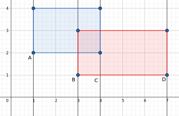
As we can see in our picture we the four lines symbolize the four steps of our line sweep. The first step (A) is to add the edge of the blue rectangle to our List of Intervals. Moreover is important that the edge also carries a reference to our rectangle. Then, in our second step (B), we add the edge of our red rectangle to our List. While adding it, we notice that there is already an edge in our list. Therefore we compare the two rectangles with each other and calculate their overlap if it exists.

4.3. An Example – Removing Rectangles

Furthermore, in our third step (C), we encounter an endpoint of our blue interval. This simply means we remove its edge from our list. Finally (D), we do the same with the edge of the red rectangle in the last step.

4.4. Implementation

algorithm LineSweep(l):
    // INPUT
    //    l = a list of rectangles
    // OUTPUT
    //    a = the area of their overlap

    a <- 0
    cList <- all x-coordinates from the rectangles
    //each x-coordinate has a reference to its rectangle
    
    n <- the length of cList

    for i <- 0 to n:
        if cList[i] = cList[i].Rectangle.left:
            m <- the lenght of cList
            for j <- 0 to m:
                a <- a + Compare(l[i], cList[j])
            cList.Add(l[i])
        else:
            cList.Remove(l[i].Rectangle)

    return a

Again we use our function “Compare” from section 3 in our for-loop.

5. Optimization and Complexity

In our first method, we compare every rectangle with each other. Thus the algorithm has complexity, where is the number of rectangles. When using the Line Sweep Method, we are still left with a time complexity. So what can we do to reduce the complexity even further?

Since we cannot simplify the “sweeping” further, our only chance is to optimize the data structure we save the rectangles in. For this purpose, we use a Binary Search Tree (BST) to save the intervals we obtained by the sweep. A so-called Interval Tree. An Interval Tree allows us to insert and delete the rectangles in . For this, we simply have to change the underlying data structure of the in our pseudocode. This leads to a complexity of with being the number of rectangles.

6. Conclusion

In this article, we discussed two ways of calculating the overlap of a set of rectangles. When we first encountered the problem, we used a very simple but costly algorithm. Our second approach uses the method of “sweeping” to reduce our two-dimensional problem to a one-dimensional one. Additionally, we reduced our complexity with the help of an Intervall Tree.