Fibonacci: Top-Down vs Bottom-Up Dynamic Programming

1. Introduction

In this tutorial, we’ll look at three common approaches for computing numbers in the Fibonacci series: the recursive approach, the top-down dynamic programming approach, and the bottom-up dynamic programming approach.

2. Fibonacci Series

The Fibonacci Series is a sequence of integers where the next integer in the series is the sum of the previous two.

It’s defined by the following recursive formula: .

There are many ways to calculate the term of the Fibonacci series, and below we’ll look at three common approaches.

2.1. The Recursive Approach

To compute in the recursive approach, we first try to find the solutions to and . But to find , we need to find and . This continues until we reach the base cases: and .

In the image below, we can see a tree of subproblems we need to solve in order to get :

One drawback to this approach is that it requires computing the same Fibonacci numbers multiple times in order to get our solution.

Let’s see if we can get rid of this redundant work.

2.2. The Top-Down Approach

The first dynamic programming approach we’ll use is the top-down approach. The idea here is similar to the recursive approach, but the difference is that we’ll save the solutions to subproblems we encounter.

This way, if we run into the same subproblem more than once, we can use our saved solution instead of having to recalculate it. This allows us to compute each subproblem exactly one time.

This dynamic programming technique is called memoization. We can see how our tree of subproblems shrinks when we use memoization:

2.3. The Bottom-Up Approach

In the bottom-up dynamic programming approach, we’ll reorganize the order in which we solve the subproblems.

We’ll compute , then , then , and so on:

This will allow us to compute the solution to each problem only once, and we’ll only need to save two intermediate results at a time.

For example, when we’re trying to find , we only need to have the solutions to and available. Similarly, for , we only need to have the solutions to and .

This will allow us to use less memory space in our code.

3. Pseudocode

3.1. The Recursive Algorithm

For our recursive solution, we just translate the recursive formula to pseudocode:

algorithm RecursiveFibonacci(N):
    // INPUT
    //   N = a non-negative integer
    // OUTPUT
    //   The N-th Fibonacci number

    if N = 0 or N = 1:
        return N

    return RecursiveFibonacci(N - 1) + RecursiveFibonacci(N - 2)

3.2. The Top-Down Algorithm

In the top-down approach, we need to set up an array to save the solutions to subproblems. Here, we create it in a helper function, and then we call our main function:

algorithm TopDownFibonacciHelper(N):
    // INPUT
    //   N = a non-negative integer
    // OUTPUT
    //   The N-th Fibonacci number

    Array <- an array of size N + 1, initialized to zeroes

    return TopDownFibonacci(N, Array)

Now, let’s look at the main top-down function. We always check if we can return a solution stored in our array before computing the solution to the subproblem as we did in the recursive approach:

algorithm TopDownFibonacci(N, Array):
    // INPUT
    //   N = a non-negative integer
    //   Array = an integer array of size N + 1 for memoization
    // OUTPUT
    //   The N-th Fibonacci number at position

    if N = 0 or N = 1:
        return N

    if Array[N] != 0:
        return Array[N]

    Array[N] <- TopDownFibonacci(N - 1, Array) + TopDownFibonacci(N - 2, Array)

    return Array[N]

3.3. The Bottom-Up Algorithm

In the bottom-up approach, we calculate the Fibonacci numbers in order until we reach . Since we calculate them in this order, we don’t need to keep an array of size to store the intermediate results.

Instead, we use variables and to save the two most recently calculated Fibonacci numbers. This is sufficient to calculate the next number in the series:

algorithm BottomUpFibonacci(N):
    // INPUT
    //   N = a non-negative integer
    // OUTPUT
    //   The N-th Fibonacci number

    if N = 0 or N = 1:
        return N

    A <- 0
    B <- 1

    for I <- 2 to N:
        Temp <- A + B
        A <- B
        B <- Temp

    return B

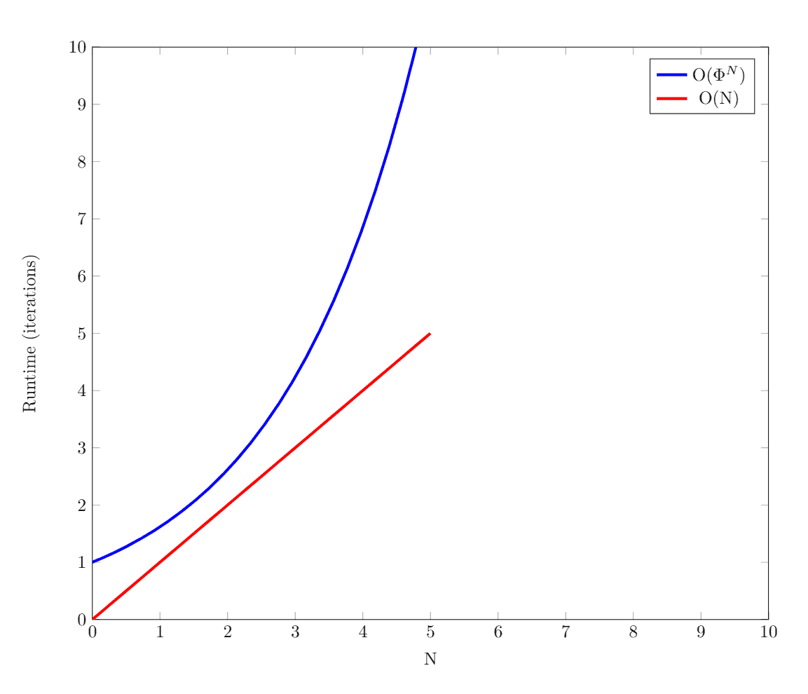
4. Complexity Analysis

The time complexity of the recursive solution is exponential – to be exact. This is due to solving the same subproblems multiple times.

For the top-down approach, we only solve each subproblem one time. Since each subproblem takes a constant amount of time to solve, this gives us a time complexity of . However, since we need to keep an array of size to save our intermediate results, the space complexity for this algorithm is also .

In the bottom-up approach, we also solve each subproblem only once. So the time complexity of the algorithm is also . Since we only use two variables to track our intermediate results, our space complexity is constant, .

Here’s a graph plotting the recursive approach’s time complexity, , against the dynamic programming approaches’ time complexity, :

5. Conclusion

In this article, we covered how to compute numbers in the Fibonacci Series with a recursive approach and with two dynamic programming approaches.

We also went over the pseudocode for these algorithms and discussed their time and space complexity.