

Learn through the super-clean Baeldung Pro experience:
>> Membership and Baeldung Pro.
No ads, dark-mode and 6 months free of IntelliJ Idea Ultimate to start with.
Last updated: March 18, 2024
Learn through the super-clean Baeldung Pro experience:
>> Membership and Baeldung Pro.
No ads, dark-mode and 6 months free of IntelliJ Idea Ultimate to start with.
In this article, we’ll implement two common algorithms that evaluate the nth number in a Fibonacci Sequence. We’ll then step through the process of analyzing time complexity for each algorithm.
Let’s start with a quick definition of our problem.
The Fibonacci Sequence is an infinite sequence of positive integers, starting at 0 and 1, where each succeeding element is equal to the sum of its two preceding elements.
If we denote the number at position n as Fn, we can formally define the Fibonacci Sequence as:
Fn = o for n = 0
Fn = 1 for n = 1
Fn = Fn-1 + Fn-2 for n > 1
Therefore, the start of the sequence is:
0, 1, 1, 2, 3, 5, 8, 13, …
So, how can we design an algorithm that returns the nth number in this sequence?
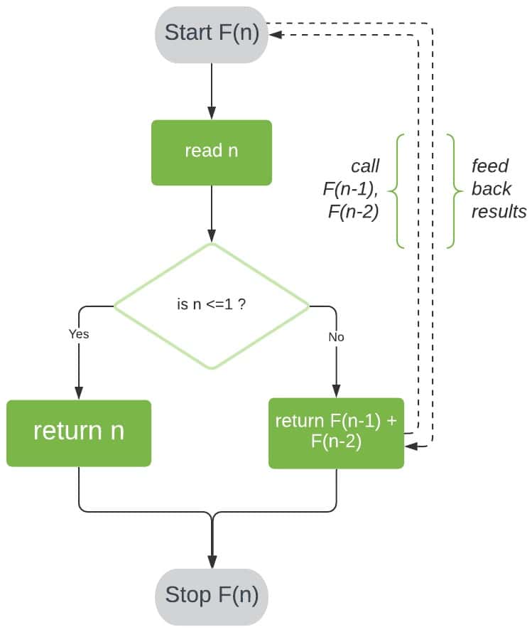
Our first solution will implement recursion. This is probably the most intuitive approach, since the Fibonacci Sequence is, by definition, a recursive relation.
Let’s start by defining F(n) as the function that returns the value of Fn.
To evaluate F(n) for n > 1, we can reduce our problem into two smaller problems of the same kind: F(n-1) and F(n-2). We can further reduce F(n-1) and F(n-2) to F((n-1)-1) and F((n-1)-2); and F((n-2)-1) and F((n-2)-2), respectively.
If we repeat this reduction, we’ll eventually reach our known base cases and, thereby, obtain a solution to F(n).
Employing this logic, our algorithm for F(n) will have two steps:
Here’s a visual representation of this algorithm:
Now that we understand how this algorithm works, let’s implement some pseudocode:
algorithm F(n):
    // INPUT
    //    n = Some non-negative integer
    // OUTPUT
    //    The nth number in the Fibonacci Sequence
    if n <= 1:
        return n
    else:
return F(n - 1) + F(n - 2)We can analyze the time complexity of F(n) by counting the number of times its most expensive operation will execute for n number of inputs. For this algorithm, the operation contributing the greatest runtime cost is addition.
Let’s use T(n) to denote the time complexity of F(n).
The number of additions required to compute F(n-1) and F(n-2) will then be T(n-1) and T(n-2), respectively. We have one more addition to sum our results. Therefore, for n > 1:
T(n) = T(n-1) + T(n-2) + 1
When n = 0 and n = 1, no additions occur. This implies that:
T(0) = T(1) = 0
Now that we have our equation, we need to solve for T(n).
There are several ways we could do this. We’ll implement a fairly straightforward approach, where we slightly simplify T(n) and find its solution using backward substitution. The result will give us an upper bound on the time complexity of T(n).
Let’s start by assuming that T(n-2) ≈ T(n-1). Don’t worry about why just yet – this will become apparent shortly.
Substituting the value of T(n-1) = T(n-2) into our relation T(n), we get:
T(n) = T(n-1) + T(n-1) + 1 = 2*T(n-1) + 1
By doing this, we have reduced T(n) into a much simpler recurrence. As a result, we can now solve for T(n) using backward substitution.
To do this, we first substitute T(n-1) into the right-hand side of our recurrence. Since T(n-1) = 2*T(n-2) + 1, we get:
T(n) = 2*[2*T(n-2) + 1] + 1 = 4*T(n-2) + 3
Next, we can substitute in T(n-2) = 2*T(n-3) + 1:
T(n) = 2*[2*[2*T(n-3) + 1] + 1] + 1 = 8*T(n-3) + 7
And once more for T(n-3) = 2*T(n-4) + 1:
T(n) = 2*[2*[2*[2*T(n-4) + 1]+ 1] + 1] + 1 = 16*T(n-4) + 15
We can see a pattern starting to emerge here, so let’s attempt to form a general solution for T(n). It appears to stand that:
T(n) = 2k*T(n–k) + (2k-1)
For any positive integer k. We can prove this equation holds through simple induction – for brevity’s sake, we’ll skip this process.
Finally, we can find k and, thereby, solve T(n), by substituting in T(0) = 1.
For T(0), we can see that n – k = 0. Rearranging, we get k = n. Now, substituting in our values for T(0) and k, we get:
T(n) = 2n*T(0) + (2n-1) = 2n + 2n – 1 = O(2n)
Recall the assumption we made earlier that T(n-2) ≈ T(n-1). Since T(n-2) ≤ T(n-1) will always hold, our solution O(2n) is an upper bound for the time complexity of F(n).
It does not, however, give us the tightest upper bound. Our initial assumption removed a bit of precision. The tightest upper bound of F(n) works out to be:
T(n) = O(Φn)
Where Φ = (1+√5) / 2.
Both of these solutions reveal that the run time of our algorithm will grow exponentially in n. This observation is quite intuitive if we consider that each time we call F(n), it will potentially make two more calls to F, thus doubling the cost of F(n). This is some very undesirable behavior!
Let’s move on to a much more efficient way of calculating the Fibonacci Sequence.
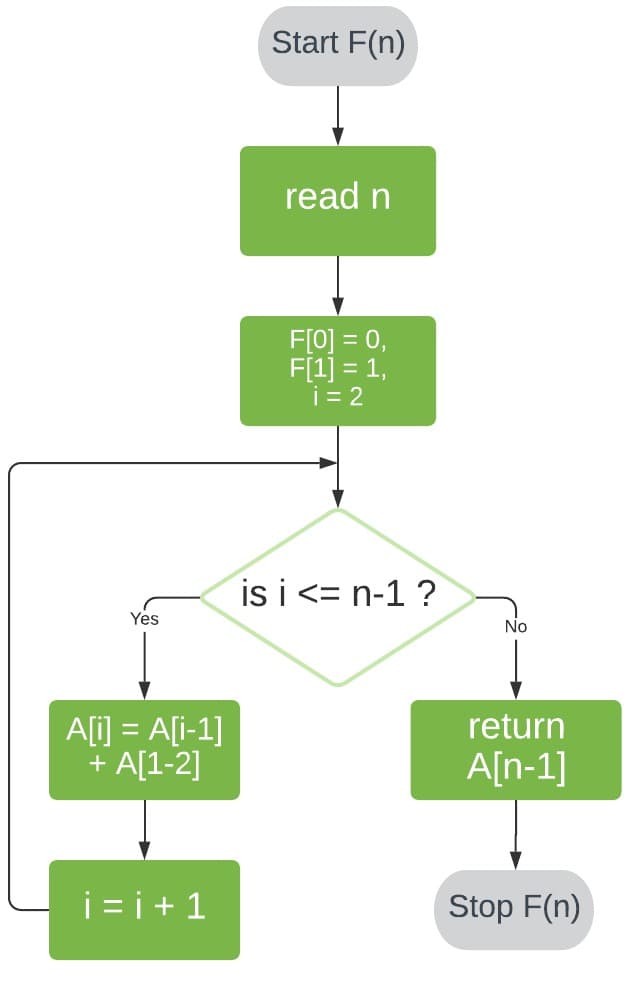
For this algorithm, we’ll start at our known base cases and then evaluate each succeeding value until we finally reach the nth number. We’ll store our sequence in an array F[].
First, we’ll store 0 and 1 in F[0] and F[1], respectively.
Next, we’ll iterate through array positions 2 to n-1. At each position i, we store the sum of the two preceding array values in F[i].
Finally, we return the value of F[n-1], giving us the number at position n in the sequence.
Here’s a visual representation of this process:
Let’s take a look at the pseudocode for this approach:
algorithm F(n):
    // INPUT
    //    n = Some non-negative integer
    // OUTPUT
    //    The nth number in the Fibonacci Sequence
    A[0] <- 0
    A[1] <- 1
    for i <- 2 to n - 1:
        A[i] <- A[i - 1] + A[i - 2]
return A[n - 1]Analyzing the time complexity for our iterative algorithm is a lot more straightforward than its recursive counterpart.
In this case, our most costly operation is assignment. Firstly, our assignments of F[0] and F[1] cost O(1) each. Secondly, our loop performs one assignment per iteration and executes (n-1)-2 times, costing a total of O(n-3) = O(n).
Therefore, our iterative algorithm has a time complexity of O(n) + O(1) + O(1) = O(n).
This is a marked improvement from our recursive algorithm!
In this article, we analyzed the time complexity of two different algorithms that find the nth value in the Fibonacci Sequence. First, we implemented a recursive algorithm and discovered that its time complexity grew exponentially in n.
Next, we took an iterative approach that achieved a much better time complexity of O(n).